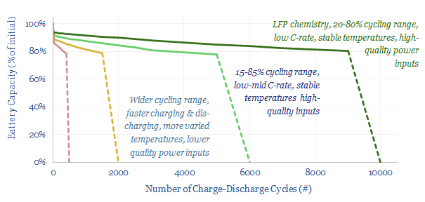
What causes battery degradation? This 14-page note offers five rules of thumb to maximize the longevity of lithium-ion batteries, in grid-scale storage and electric vehicles. The data suggest hidden upside in the demand for batteries, for lithium and high-quality power electronics, especially if batteries are to backstop renewables.
Battery degradation matters. Small changes in battery modelling parameters — e.g., a 3-4% decline rate and a 2-3 year shorter lifespan — can obliterate a 10% IRR on a grid-scale battery. Conversely, optimizing the lifespan and functioning of a battery can double its IRR (page 2).
We present a very simple “rule of thumb” model on page 3. Then we explain why batteries degrade on pages 4-5, covering fabled mechanisms such as the solid electrolyte interface, lithium plating, positive electrode decomposition, particle fracturing. In total there are 18 main battery degradation pathways.
The complexity gets worse. We aggregated 7M data-points into a big battery degradation data file, in turn sourced from excellent lab studies by Sandia National Laboratories. When the exact same cells are tested under the exact same cycles, their lifespans can vary by a factor of 3x. One of the drivers of degradation is random manufacturing defects (page 6).
Five rules of thumb for battery degradation may nevertheless be helpful, to derive actionable conclusions. The top five drivers of battery degradation are reviewed on pages 7-11. In each case, we outline the parameter, why it causes degradation, and how it can be improved.
Are lithium ion batteries a good fit for backing up volatile renewables inputs? We answer this question on pages 12-13. There is an array of companies that increasingly excites us here, such as CATL, Stem, Powin, Eaton, supercapacitors, and other power electronics names; and general upside for lithiumdemand, as degradation can best be avoided by over-sizing the batteries.
However, we also fear some battery projects may end up underwater and we see more muted upside for metals such as nickel and cobalt, due to the degradation rates of different battery chemistries, which does seem to favor LFP.
Data and details on what causes battery degradation are in the note, alongside a more actionable overview of maximizing battery value.
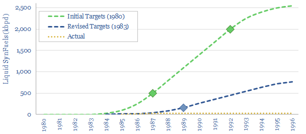
Does policy de-risk new technology? This 10-page note is a case study. The Synthetic Fuels Corporation was created by the US Government in 1980. It was promised $88bn. But it missed its target to unleash 2Mbpd of next-generation fuels by 1992. There were four challenges. Are they worth remembering in new energies today?
The Synthetic Fuels Corporation was created by the US Government in 1980. To great fanfare. Its goal was unleashing synfuels. At $325bn in today’s money, its budget was actually quite similar to the energy-climate portion of 2022’s Inflation Reduction Act.
We explore other similarities between energy policies in the 1980s, the creation of the SFC, and emerging policies in the energy transition (pages 2-4). Our conclusion is that the similarities are surprisingly striking.
The main production pathway that was envisaged in the creation of synfuels started with coal, produced hydrogen as an intermediate, and then converted syngas into liquid fuels. The process is described in more detail on page 5.
Costs are a challenge. We have modelled the energy costs of synfuels, in today’s money, using models of coal gasification and gas-to-liquids. Ultimate costs of synfuels — in $/bbl and c/kWh-th — are derived on page 6.
Efficiency is a challenge. We modelled the thermodynamics and energy penalties of producing synfuels, in a helpful waterfall chart schematic on page 11. You cannot get around the second law of thermodynamics.
Other technical challenges are discussed on page 8. Some projects backed by the SFC simply did not work. Others were very small scale (around 5kbpd).
Politics could be described as the biggest barrier. Policies have an annoying habit of changing. The downfall of the US’s political push towards synfuels, which played out throughout the 1980s, is summarized on page 9.
Does policy de-risk new technology? We draw out conclusions for the energy transition on page 10. We all clearly want to avoid repeating mistakes of the 1980s. So our goal is to offer constructive suggestions for decision-makers, investors and project developers.
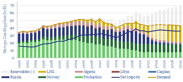
Modelling Europe’s gas balances currently feels like grasping at straws. Yet this 10-page note makes five predictions through 2030. Thus our new European gas outlook revises our views on how fast new energies ramp, which gas gets displaced first, which energy sources are no longer ‘in the firing line’, and how gas pricing will evolve from here.
Our starting point for understanding Europe’s gas market in 2022 to 2030 is to consider the ramp up of new energies. We see enough growth from wind and solar to displace the equivalent of 14 bcfd from Europe’s 45bcfd gas market by 2030 (page 2).
Who is in the firing line to be displaced? Russia’s gas supplies to Europe are discussed on page 3, including our latest gas supply modelling.
Who is no longer in the firing line? If the ramp up of renewables primarily displaces Russian gas, then we would need to upgrade our estimates for indigenous European gas production, coal consumption, nuclear generation, uranium consumption and LNG imports. The numbers are quite interesting and material, spelled out on page 4.
But timing matters. The ramp up of renewables is gradual. Conversely, Russian supplies could be offline through 2023, 2024. A 3-10bcfd gas shortage in Europe may persist through 2025, 2026. The moving pieces are described on pages 5-6.
Our pricing outlook is that 2023, 2024 could be worse than 2022. We think gas prices can continue making new highs for as long as policymakers continue to subsidise gas and cushion against demand destruction. Some numbers, in $/mcf, are thrown around on page 7-8.
Ultimately policymakers may need to change tack, and act to reduce demand. The higher gas prices go in 2023, 2024, then the more likely this will happen. Our European gas outlook, pricing scenario, and possible ‘rationing options’, are spelled out on pages 9-10.
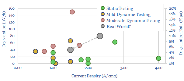
What degradation rate is expected for a green hydrogen electrolyser, if it is powered by volatile wind and solar inputs? This 15-page note reviews past projects and technical papers. 5-10% pa degradation rates would raise green hydrogen costs by $1/kg. Avoiding degradation justifies higher capex, especially on power-electronics and even batteries?
The second-by-second output from renewables is volatile. The volatility of solar includes around 100 volatility events per day. The volatility of wind includes around 75 volatility events per day. This is usually fine, as it can be smoothed out in large and diversified power grids, or via different batteries (pages 2-3).
But how can electrolysers run off renewables? This feels like an increasing necessity for green hydrogen, in order to ensure the hydrogen has minimal embedded CO2, and under new requirements from the US Inflation Reduction Act (page 4).
Degradation of electrical equipment under volatile input feeds, including case studies from the motor industry, are reviewed on (page 5).
A brief history of electrolyser and PEM fuel cell deployments are reviewed, in order to draw conclusions on the decline rates of installed systems (pages 6-7).
The technical literature into PEM electrolyser degradation is then reviewed on pages 8-10. We think uncertainty is still high, and it would be helpful to conduct more studies, longer studies and more rugged studies into electrolyser degradation under volatile inputs.
A case study is drawn from the technical literature and described in detail, explaining how dynamic loading has been linked to the degradation of electrolysers. Total stoppages of electrolysers may be a driver of degradation, and require further back-ups (pages 11-13).
Economic implications are spelled out on page 14. As a rule of thumb, adding a 5% pa decline rate to a base case electrolyser model might raise the total levelized cost of hydrogen by around $1/kg.
Can electrolysers run off renewables? Ultimately our answer to this question is yes, but it may require adding power electronics and batteries alongside the electrolysers, in a trade off with up-front capex, in order to mitigate against degradation.
Our roadmap to net zero still sees relatively more potential in large-scale transmission infrastructure, and short-duration battery back-ups, in order to maximize the ascent and impact of renewables.
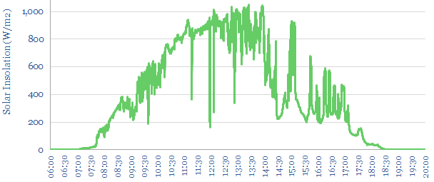
This 20-page note quantifies the statistical distribution of the short-term volatility of solar power plants, by evaluating second-by-second data, for an entire year. Solar output typically flickers downwards by over 10%, around 100 times per day. We want to ramp solar in the energy transition. But how can industrial processes truly be ‘powered by solar’? Buffering the volatility creates opportunities for gas and nuclear back-ups, inter-connectors, supercapacitors, smart energy and power electronics?
Fleetwood Mac released their classic hit, ‘Little Lies’, in the winter of 1987. In the song, Christine McVie describes a once-wonderful relationship that has ultimately run its course. There is a reluctance to accept this fact about the future. Hence the song’s chorus pleads “tell me lies, tell me sweet little lies”. The refrain is then hauntingly echoed by Stevie Nicks and Lindsey Buckingham (“tell me, tell me lies!”).
This research note is a statistical analysis of an entire year’s second-by-second solar volatility (our methodology is laid out on pages 2-5). It is a nerdy and numerical topic. Hence without wishing to dilute the importance of this issue, we are going to draw some inspiration from Fleetwood Mac in our chapter headings.
For example, should solar power keep ramping up forever, to over 50% of future power grids? Or might solar slow down, after running its course, and ramping to 20-30%? And are analysts like us, who want to see solar capacity additions ramp up by 3-5x in the energy transition, wilfully asking to be told sweet little lies about overcoming short-term volatility issues? Our goal is to use data and find genuine, objective answers to these questions.
Variability. The best day, a typical day and the worst day of second-by-second solar volatility are presented on pages 6-9. For example, the chart above shows the second-by-second solar output at a typical-good day, with relatively little short-term volatility.
The statistical distribution of different days’ solar volatility is plotted in candlestick charts and marimekko charts on pages 10-11. There is volatility in the volatility itself.
“Powered by solar”. Can we power typical industrial processes purely from input feeds like the ones we have shown in our chart above, and throughout this report? Issues that need to be overcome are discussed on pages 12-15. They include annoyingness, lost output, mission-critical loads, damaged work-in-progress and faster degradation rates at industrial machinery.
Overcoming volatility. We want to ramp solar as much as possible as part of our ‘roadmap to net zero‘. We think a future grid with 20-30% solar are optimal, which involves a 3-5x acceleration in the pace of annual solar deployments. However, smoothing the short-term volatility, we think, is also going to create concomitant opportunities (page 16).
The best opportunities to de-bottleneck short-term solar volatility include diversified and resilient power grids, gas and nuclear back-ups, super-capacitors, inter-connectors, smart-energy, demand shifting and power electronics. The merits, drawbacks and costs (in $/kW) of these different solutions are presented on pages 17-20.
This note into the short-term volatility of solar (i.e., second-by-second) aims to complement our other research into the long-term volatility of solar (i.e., year-by-year). It is interesting that building out power grids and inter-connectors helps to resolve both issues.
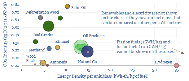
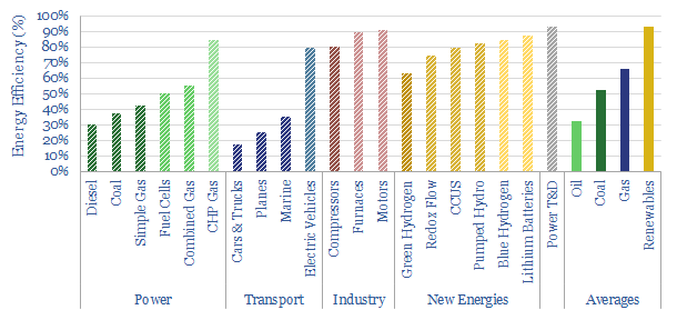
Energy is the glue of our universe. Literally everything is at some level an energy flow – from viewing this text to matter itself – which can be expressed in Joules and kWh. Hence this 16-page overview is a useful reference, to translate from any energy units to any others; for comparisons; and to understand the units in energy transition.
This reference document is an attempt to condense 15-years of energy research into a single overview, for anyone wishing to understand energy from first principles, juggle energy units seamlessly, and compare different energy technologies.
We will consider it ‘mission accomplished’ if this document gets printed, earns its keep on the desks of energy analysts for the foreseeable future; and despite the complex, numerical topic, if it leaves readers in awe of energy and vaguely amused by some of the ‘fun facts’.
Energy is the glue of our universe, and everything that happens within it: making things warmer, cooler, faster, slower, bigger, smaller, visible, audible, electrically charged, or chemically changed. Thus the ‘Joule’ is a miraculous unit, which definitionally links electricity, heat, motion, physics and chemistry, as explained on page 2.
However the kWh is a more useful unit, because 40% of all global energy is electricity, which in turn is primarily metered, bought and sold in kWh (or MWH). Our advice to understand energy transition is to translate everything into kWh (page 3).
An intuitive guide to mastering the orders of magnitude, from kWh to thousands of TWH, is presented on pages 4-5. This includes electrical processes, producing materials and entire countries’ energy balances.
Primary energy versus useful energy is another crucial distinction. Primary energy denotes the thermal energy contained in the bond enthalpy of fuels (yes, we will explain this in a way that is intelligible and avoids unnecessary jargon). But only a portion of this energy can be harnessed as useful energy, due to efficiency losses (page 6-8).
A reference for gas industry units is given on pages 9-10, converting gas units into kWh from standard cubic feet (mcf, mmcf, bcf, TCF), normal cubic feet, cubic meters, tons of gas, tons of LNG (MT, MTpa), British thermal units, the archaic therm; higher heating value versus lower heating value, and real-world gas blends. Gas is a low-carbon fuel as 54% of gas energy comes from converting hydrogen (in CH4) into water vapor.
A reference for oil industry units is given on page 11, converting oil units into kWh from gallons, barrels (bbls, kbbls, Mbbls, bn bbls), boe (boe, kboe, Mboe, bn boe), kilograms and tons; for ethane, methanol, ethanol, propane, butane, octane, gasoline, jet fuel, diesel, fuel oil and the ‘blended average oil barrel’; and the CO2 intensity of oil, of all of the above.
A reference for coal industry units is given on page 12, converting coal units into kWh from tons (kTpa, MTpa, GTpa), and the associated CO2 intensity of coal. The key challenge is understanding different coal grades, from anthracite, to bituminous, to sub-bituminous, to lignite.
A reference for biomass industry units is given on page 13, converting wood fuels into kWh from wet tons, dry tons, and across different products, such as fresh wood, dry wood, deforestation wood, wood chips, briquettes, wood pellets, charcoal.
A reference for food energy units is given on page 14, converting from calories into kWh, for different food products, within the world’s 10GTpa food production. The drawback of the calorie, as a unit of energy is an annoying custom, that many commentators abbreviate kiloCalories as ‘Calories’. This makes many technical papers confusing. It would be as though somewhat decided that ‘dollars’ would be a really handy abbreviation for ‘1,000 dollars’, and then sent you haphazardly into a casino.
A reference for hydrogen units is given on page 15, converting from kg of hydrogen into kWh, both in higher heating value and lower heating value terms, and for different volumes of hydrogen at standard conditions, for liquid hydrogen at -253C, and for compressed hydrogen at 10,000 psi. It is interesting to compare this with natural gas.
Other fuels and comparisons are also covered on pages 16-17. An amazing fact is that 1 kg of hydrogen releases 3 million times more energy as a fusion fuel than a combustion fuel. We also discuss the first and second laws of thermodynamics, which matters for maximizing the efficiency of clean fuels.
The note ends with some reference tables and links to our other data-files. Another excellent and free resource for comparing different fuels is Engineering Toolbox. We hope our own note is helpful for understanding all of our energy transition research.
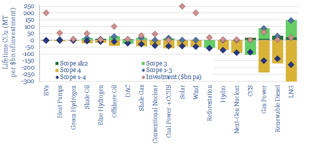
Scope 4 CO2 emissions reflect the CO2 avoided by an activity. This 11-page note argues the metric warrants more attention. It yields an ‘all of the above’ approach to energy transition, shows where each investment dollar achieves most decarbonization and maximizes the impact of renewables.
Scope 1-3 CO2 emissions are now familiar to most decision-makers. Scope 1 captures the CO2 emitted directly in creating a product. Scope 2 adds the CO2 emitted in generating electricity used to create the product. And Scope 3 adds the CO2 emitted in using the product, for example, by combusting it. A summary is presented by fuel and by material on pages 2-3, with the implication that ‘everything is bad, only some things are less bad than others’.
Scope 4 CO2 is intended as an antidote to the depressed conclusion that ‘everything is bad’. It considers the CO2 avoided by an activity. Working from home avoids the CO2 of a commute. Building a wind farm may displace CO2-intensive coal. So too might developing a gas field. Thus the purpose of this note is to construct Scope 1-4 CO2 calculations for 20 different energy technologies, fairly, objectively, and then draw conclusions. The numbers are remarkable (page 4).
‘All of the above’. Every single option in our chart above has net negative Scope 1-4 CO2 emissions. The more investment that flows in to all of these categories, the faster the world will decarbonize. Our overall roadmap to net zero needs to treble global energy capex to over $3trn pa (pages 4-8).
Project developers and investors should consider Scope 4 CO2. Many categories with deeply negative Scope 1-4 CO2 emissions — sometimes achieving 3x more net CO2 abatement per $1bn of investment than wind, solar and EVs — have been unsuccessful in attractive capital. It may therefore be appealing for project-developers to present Scope 1-4 CO2 benefits on a clear and transparent basis. It may also be appealing for investors to communicate the Scope 1-4 CO2 of their portfolios to their own stakeholders (page 9).
Maximizing decarbonization. Scope 4 CO2 emissions depend on counterfactuals. What is an activity displacing? This matters across the board and can also promote faster decarbonization. For example, a new wind project that displaces nuclear achieves no net decarbonization, whereas an inter-connector that allows that same wind project to displace coal-power avoids 1.2 kg/kWh of CO2 (page 10).
Conceptual limitations of Scope 4 CO2 are discussed on page 11. However, we conclude it is an increasingly important metric for decision makers in the energy transition, to ensure adequate energy supplies are developed, while also decarbonizing as fast as possible.
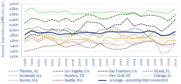
The solar energy reaching a given point on Earth’s surface varies by +/- 6% each year. These annual fluctuations are 96% correlated over tens of miles. And no battery can economically smooth them. Solar heavy grids may thus become prone to unbearable volatility? Our 17-page note outlines this important challenge, and finds that high-voltage interconnectors cure renewables volatility most effectively. It also helps to keep power grids diversified.
Renewables incur volatility over different timeframes, from second-to-second to year-by-year. We outline the most effective solution to each volatility duration on page 2. But year-by-year volatility is most challenging…
How bad is it? We have aggregated data from the excellent NREL NRRDB resource, showing the average solar energy arriving at ten major cities, hour-by-hour, for 23-years. The average location sees +/- 6% annual volatility in the solar energy reaching ground level, as quantified and discussed on pages 3-5.
What implications for energy supplies? A future energy system relying on solar for 50% of its incoming energy would therefore appear to incur comparable annual supply volatility to Saudi Arabia’s entire oil supplies vanishing from the market every year, then magically returning the next year. Or similar to Japan having to accommodate the Fukushima nuclear crisis every other year. Or Europe having to accommodate a shut off of 25% of Russia’s gas every other year. One cannot help wondering whether this would connote very large energy price volatility or indeed whether we have already entered this era (page 6).
Can batteries offer a solution? We explore this option on page 7. The maths simply do not work and the numbers get very silly very quickly.
Can wind offer a solution? We explore this option on pages 8-9. The answer is partially. Although wind speeds also vary year-by-year, and sometimes cross-correlate with solar.
Can power transmission lines offer a solution? We explore this option on pages 10-16, including some deep-dive modelling. The results are fascinating. Annual solar volatility is 96% correlated within an individual city, 50-70% correlated with neighboring cities, but completely non-correlated with other regions on the Continent. A single 2.5 GW inter-Continental transmission line that smooths out two 10 GW+ solar-heavy regions can effectively halve their annual volatility. We think up-scaling HVDCs is the best option to achieve resilient and renewable-heavy power grids. Numbers and costs are quantified. But overall, we conclude that interconnectors cure renewables volatility.
Can diversified power grids offer a solution? Our modelling also suggests that resilient grids should retain a healthy mix of supply sources, including wind, nuclear, hydro, and gas (the latter paired with CCUS or nature-based CO2 removals). Conclusions are on page 17, the full notes can be downloaded below, and underlying data-models can be audited here and here.
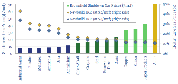
Dispersion in global gas prices has hit new highs in 2022. Hence this 17-page note evaluates two possible solutions. Building more LNG plants achieves 15-20% IRRs. But displacing industrial gas demand in Europe, then re-locating it in gas-rich countries can achieve 20-40% IRRs, lower net CO2 and lower risk? Both solutions should step up. What implications?
Global gas price dispersion is hitting new highs, with the best geographies remaining consistently below $2.5/mcf, but many others spiking to peak prices in 2022. Theories of gas price dispersion are laid out on pages 2-3, while we present data and conclusions on 20 different countries’ gas prices on pages 4-6.
Will it accelerate renewables? An interesting observation is that the countries with spiking gas prices are already deploying renewables ‘as fast as feasible’. Whereas it is often the countries with very low gas prices that have very low renewables deployment (page 7).
Will it accelerate LNG? In theory yes. Our expectations for future gas prices should unlock 15-20% IRRs at new LNG projects, and our growth forecasts are on page 8.
Will it accelerate industrial re-location, away from geographies with high-priced gas, and towards geographies with low-cost gas. This is the main focus of the note. And we think greenfield industrial facilities can earn 20-40% future IRRs if they are sited in geographies with low-priced gas. By contrast, we have constructed a ‘shutdown curve’ showing what gas prices are needed to free up 13bcfd of industrial gas demand in Europe. Our modelling framework is explained on pages 10-12.
There are further economic and ESG advantages to re-locating industry to gas-rich countries, compared with exporting their gas. They are quantified on pages 13-14.
Who benefits? We outline examples of leading companies in gas-rich countries on pages 15-16. This includes both emerging world producers, US E&Ps and US industrial companies that have featured in our research to-date.
Finally, for the renewables and LNG industries, we would highlight that this analysis is not an either-or. We will need all solutions to alleviate energy shortages. Yet displacing industrial gas demand in Europe may mute the kind of runaway cost-inflation that de-railed the LNG industry in the 2010s, and threatens the renewables industry in the 2020s (page 17).
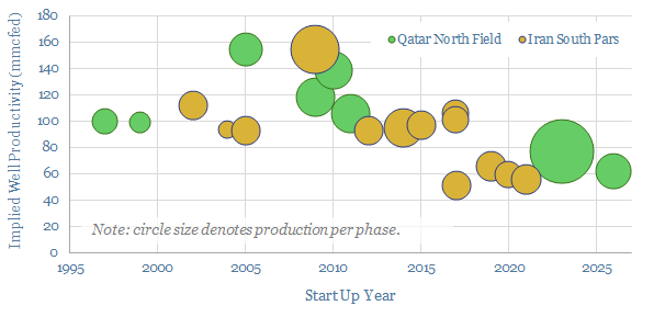
North Field gas production is now the most important conventional energy source on the planet. It produces 4% of world energy, 20% of global LNG and aims to ramp another 50MTpa of low-carbon LNG by 2028. But what if Qatar’s exceptional reliability gets disrupted by unforeseen conflict with Iran? Without wishing to catastrophize, this 18-page note on the North Field energy production explores important tail-risks for near-term energy balances and long-term energy transition.
There is no slack in the system for LNG outages in 2022-26. Our global energy balances, gas balances, and the ‘hole’ left by possible Russian gas supply disruptions are quantified on pages 2-4.
Thus the Qatari North Field is now the most important conventional gas field in the world. It underpins 20% of global LNG. And as it straddles the Iranian border, the combined output from the field equates to 4% of all useful energy on the planet (equivalent to all of the world’s wind and solar assets combined) (pages 5-6).
And it is being expanded, adding another 50MTpa of low-carbon LNG to quell LNG under-supply in the mid-late 2020s, which helps advance energy security and global decarbonization (pages 7-9).
But what if this enormous field were to disappoint in some way? Its historical reliability has been exceptional. However, without wishing to catastrophize, there is now evidence of intensifying resource competition between Qatar and Iran causing well productivities to decline at the field. We have aggregated data from technical papers and press reports on pages 10-13.
Or worse. Iran is literally designated as the world’s leading State sponsor of terrorism by the US government. It has a fraught historical relationship with the West, with the GCC and with Qatar. It has funded drone attacks on Saudi oil infrastructure. Vladimir Putin visited Iran in July-2022, to discuss greater cooperation. Again, without wishing to catastrophize, this warrants some objective analysis over tail risks (pages 14-17).
Our conclusions, for energy markets and energy transition, are laid out on pages 17-18. A resilient energy system will need to be well diversified, including a buffer of excess capacity, if the world seeks to decarbonize without excessive risks.
Underlying data on North Field gas production and productivity is linked here.
Cookies?
This website uses necessary cookies. Our cookies are simply to improve your experience. We do not undertake any advertising or targeting via our cookies. By clicking 'accept' or continuing to use the website, you consent to our use of cookies.AcceptRead More
Privacy & Cookies Policy
Privacy Overview
This website uses cookies to improve your experience while you navigate through the website. Out of these, the cookies that are categorized as necessary are stored on your browser as they are essential for the working of basic functionalities of the website. We also use third-party cookies that help us analyze and understand how you use this website. These cookies will be stored in your browser only with your consent. You also have the option to opt-out of these cookies. But opting out of some of these cookies may affect your browsing experience.
Necessary cookies are absolutely essential for the website to function properly. This category only includes cookies that ensures basic functionalities and security features of the website. These cookies do not store any personal information.
Any cookies that may not be particularly necessary for the website to function and is used specifically to collect user personal data via analytics, ads, other embedded contents are termed as non-necessary cookies. It is mandatory to procure user consent prior to running these cookies on your website.