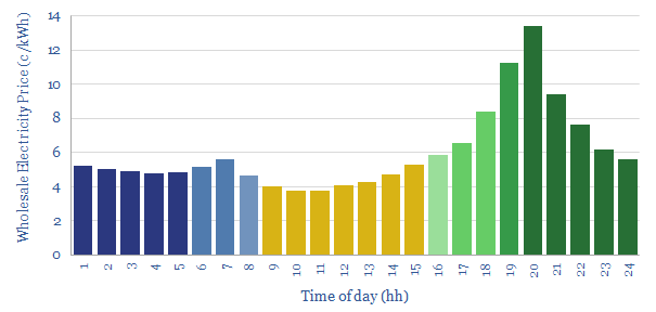
In 2023, power grids with c20-30% solar variation tend to have intra-day spreads of 9c/kWh, between peak wholesale electricity prices at 8pm and trough prices at 10am. Unusually, night-time electricity prices are 40% higher than day-time prices. This data-file quantifies California electricity prices, on a wholesale basis, at a sample of grid nodes, looking hour by hour in August-2023.
By 2023, California is generating 20% of its electricity from utility-scale solar and 10% from utility-scale wind, while the total generation from solar is as high as 30% if residential/rooftop solar is also included (EIA data here).
Hence the purpose of this data-file is to quantify the hour-by-hour volatility of power prices in a solar-heavy power grid, estimating California electricity prices by hour, using reported wholesale electricity pricing from CAISO, at individual nodes in the grid.
Across our sample of grid nodes, we find that locational marginal price has averaged 6.5 c/kWh on a wholesale basis during August-2023. The data-file also contains similar snapshots for August-2022, August-2021, August-2020, to see how intra-day power prices changed over time.
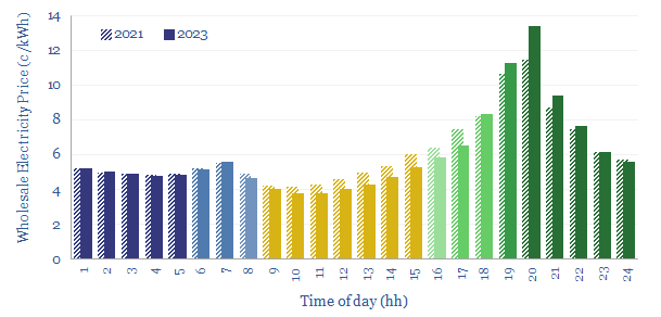
Peak and trough electricity prices? California’s lowest wholesale electricity prices are found at 10am-noon, at below 4c/kWh. California’s highest wholesale electricity prices are found at 8pm, at above 13c/kWh. Over time, there is also evidence suggesting that the curve has been getting steeper (chart below).
California IntraDay Wholesale Power Prices in 2023 and in 2021
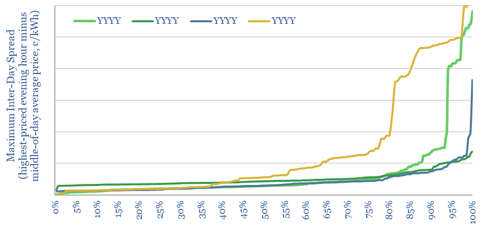
Electricity price variations by day? The data above entail that the maximum intra-day spread has recently been running at around 9c/kWh, which is lower than the 20c/kWh we think is needed for grid-scale batteries to generate attractive economic returns on storing up ‘excess’ solar during the peak of the day, and re-releasing that electricity later in the evening, after the sun has set. Although there are other more exciting roles for batteries in the near-term. For further details, please see our energy storage research.
Variability? Hour-by-hour price variations are not the same on all days, but vary vastly, with a sharp upside skew. The chart below plots the distribution of the maximum spread between each evening’s highest priced hourly power price and its prior day-time average. In theory, this is the distribution of spreads available to an intra-day battery operator.
Night versus day? Average night-time wholesale electricity pricing of 7c/kWh is now 40% higher than average day-time wholesale electricity pricing, which is somewhat unusual, as in most grids, night-time prices are lower than day-time prices. This may in turn be an argument for efficiency investment to reduce night-time electricity loads, such as efficient lighting systems.
Note that retail electricity prices are higher than wholesale prices, as they also include transmission, distribution, utility costs and taxes. At the time of writing, the latest EIA estimates are that retail electricity prices in California average 25c/kWh, including 31c/kWh for residential consumers, 24c/kWh for commercial, 19c/kWh for industrial customers, which also reminds us that overall systems can be materially higher than marginal generation costs, per our recent research note here, and all our broader power grid research.
This 14-page report re-visits our wind industry outlook. Our long-term forecasts are reluctantly being revised downwards by 25%, especially for offshore wind, where levelized costs have reinflated by 30% to 13c/kWh. Material costs are widely blamed. But rising rates are the greater evil. Upscaling is also stalling. What options to right this ship?
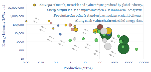
This 14-page report explores whether global industrial activity is set to become ever more concentrated in a few advantaged locations, especially the US Gulf Coast, China and the Middle East. Industries form ecosystems. Different species cluster together. Elsewhere, in our view, you can no more re-shore a few select industries than introduce dung beetles onto the moon. These mega-trends matter for economic forecasts and valuations.
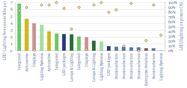
20 leading companies in LED lighting are compared in this data-file, mostly mid-caps with $2-10bn market cap and $1-8bn of lighting revenues, listed in the US, Europe, Japan, Taiwan. In 2022, operating margins averaged 8%, due to high competition, fragmentation and inorganic activity. The value chain ranges from LED semiconductor dyes to service providers installing increasingly efficient lighting systems as part of the energy transition.
The global LED industry is worth $80bn per year, with LEDs used in lighting indoor and outdoor spaces, in the automotive industry and to back-light the screens associated with the rise of the internet.
Leading companies in LED lighting range from specialists manufacturing semiconductor dyes, other specialists combining these components with other conductors and phosphors into LED packages, others encasing this product into LED lamps, others adding further drivers and housings to yield LED luminaires, and others ultimately selling entire lighting systems.
Integration versus fragmentation. Some companies are involved in the entire, integrated value chain discussed above, while others specialise in specific parts, e.g., dye/phosphor specialists upstream, or enterprise solutions businesses that design and implement overall lighting systems for corporate customers.
This data-file profiles 20 leading companies in LED lighting and the broader lighting industry. For each company, we have quantified size, recent financial metrics (e.g., revenue, operating margins), estimated exposure to the LED lighting industry and tabulated key notes. Backup tabs in the file cover LED costs, LED payback periods and LED efficiency.
Competition is high in the LED lighting industry and the average company reported an 8% operating margin in 2022.
Fragmentation is high, as the largest company in the screen derives just $7bn per annum of LED-related revenues. All 20 companies in our screen generated c$40bn of revenue in 2022.
Company sizing is therefore more skewed towards mid-cap and smaller-cap names than other company screens we have undertaken, with the larger companies in the screen having market caps in the range of $2-10bn.
Acquisition activity in the LED lighting industry has been high, and half a dozen of the companies in our screen have recently changed hands or been spun out. Details are in the data-file. For example, Philips Lighting was IPO’ed as Signify in 2016 and remains the largest integrated LED lighting company in the world.
Industry leaders in LED lighting include listed companies in the Netherlands, Japan, the US, Taiwan, China, Austria and Germany.
This data-file quantifies the energy needed to produce steam, for industrial heat, power, chemicals, CCS plants and hydrogen reforming. As rules of thumb, low pressure saturated steam at 100◦C requires 2.6 GJ/ton (720kWh/ton), medium pressure dry steam at 6-bar and 300◦C requires 3 GJ/ton (830kWh/ton) and super-critical steam at 250-bar and 600◦C requires 4 GJ/ton (1,200kWh/ton).
What is the energy content of steam at 1 atmosphere’s pressure?
At a constant pressure of 1-bar (i.e., 1 atmosphere), it takes 4.2 kJ of energy to heat each kg of water by each 1◦C (aka the specific heat capacity of water). So it might require 0.34 GJ/ton of energy to heat 20◦C water up to a boiling point of 100◦C.
Saturation point? When water in the liquid phase reaches 100◦C it becomes saturated with heat, and rather than getting hotter, additional heat will vaporize the water into steam. The resultant steam is ‘saturated steam’ in the sense that it cannot get any hotter either, until all of the water has evaporated.
Vaporizing water into steam requires breaking the bonds that hold water molecules together as a liquid, the latent heat of vaporization, which is 2,256 kJ/kg, or translated into other units, 2.3 GJ/ton.
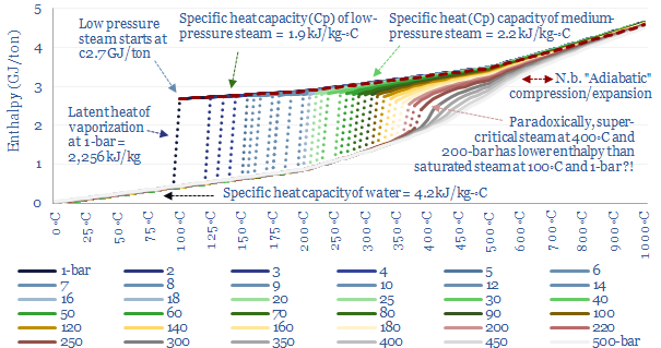
Only once all of the water has vaporized, yielding ‘dry steam’, can the temperature increase further. It takes 1.9 kJ to heat each kg of steam by each 1◦C (aka the specific heat capacity of steam, Cp). Thus the enthalpy per ton of 1-bar steam can be read off the chart below.
Specific heat of steam at 1-bar pressure starts at 2.7 GJ per ton
Units and conversions. 1 ton of steam is 1,000 kg. 1GJ is 1,000 MJ. And 1MJ is equivalent to 1,000 kJ or 0.278 kWh. For more conversions – including into tons of coal, mcf of gas, bbls of oil or alternatives such as mmbtu – please see our overview of energy units.
Amazingly, the discussion above shows that less than 20% of the thermal energy needed to make steam is the energy needed to bring room temperature water to the boil, and over 80% of the energy is needed to boil 100◦C water into 100◦C steam. This slow boiling behaviour is what allows you to cook pasta. Or at least this is the case at atmospheric pressure.
What is the energy content of pressurized steam?
The discussion above simplistically assumed 1-bar of pressure. In other words, it assumed that the steam can expand immediately when it is produced, into a wide open area.
In practice, industrial facilities will prefer to generate pressurized steam. Pressurized steam is more useful. It will naturally flow wherever you direct it, without needing to be compressed using a capex-intensive, maintenance intensive and energy-intensive compressor. But it also makes the energy economics more complicated.
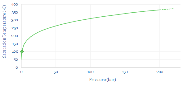
Pressure changes water’s boiling point? When water boils into steam at 1-bar of pressure, then its volume naturally expands by 1,600x. Hence if the steam is held in a closed or semi-closed vessel, the pressure will naturally start to rise very significantly. In turn, as pressure rises, the saturation temperature for water also rises. The boiling point rises. At 100-bar (i.e., 100 atmospheres of pressure), water does not boil until 300◦C.
Saturation temperature of water
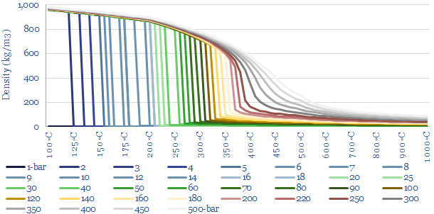
So how does this change the energy costs of making steam? You might intuitively think that it would require more energy to boil water into steam with higher temperature and pressure. But this is not entirely the case. When gases expand, they cool. And so the more they expand, the more energy must be added to heat them back up again to maintain the desired temperature. High pressure steam, by definition, has expanded less than low pressure steam. This is shown in the chart below. At 1-bar, boiling 100◦C water into 100◦C steam requires a 1,600x expansion. But boiling water at 100- bar and 500◦C only requires a 33x expansion. Generating higher density steam requires less energy to be added to ‘make up for’ the natural tendency of gases to cool down as they expand. So how can we quantify this effect?
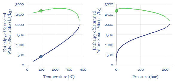
In energy terms, we can quantify how the latent heat of vaporization declines as pressure and temperature increase. At 1-bar of pressure, water boils at 100◦C, and this requires overcoming the latent heat of vaporization of water, of 2,256 kJ/kg, which is shown in the charts below as the difference between the green dot and the blue dot. But the chart also shows how the latent heat of vaporization decreases, at higher temperatures and pressures. There is ever more enthalpy in the water phase. And less energy must be re-added to compensate for the cooling effects of gas expansion.
Critical point of steam illustrated via the enthalpy of saturation steam versus temperature and pressure
What is the critical point of steam? Ultimately, there is a point on the diagram, at 220-bar and 375◦C temperature where the latent heat of vaporization has fallen to zero. This is the ‘critical point’. At 220-bar of pressure and 375◦C temperature there is effectively no difference between steam and water. There is no sudden point of expansion! Just a very hot and dense soup of water particles. Supercritical fluids, which lie above their critical temperatures and pressures, can get hotter and denser than subcritical fluids, which is useful for efficient power generation.
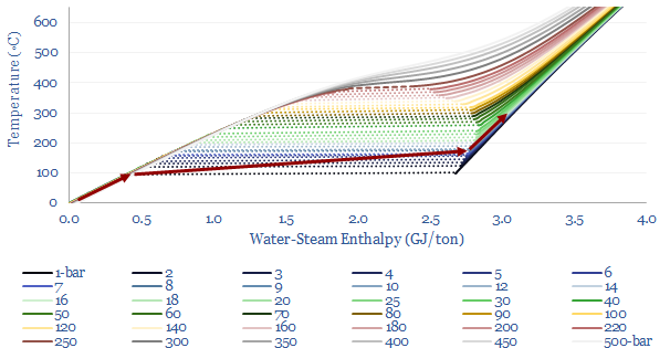
The relationship between steam’s enthalpy and temperature is plotted below, this time with more sensitivity, ranging from 0-600◦C of temperature and 1-500 bars of pressure. The solid lines illustrate specific heat, where energy is added to the fluid mixture raising its enthalpy and its temperature. The dashed lines show the latent heat of vaporization for saturated steam, where further energy must be added to vaporize water, before the temperature can increase any further. And as noted above, the latent heat of vaporization becomes smaller and smaller at higher pressures and temperatures, up to the critical point, where the latent heat of vaporization is zero.
Enthalpy of steam versus temperature in GJ per ton and C as pressure rises
For a good rule of thumb, you can read off the enthalpy of steam from this chart, depending on its temperature and pressure.
You can also compare the energy content of steam at different temperatures and pressures using the chart above, to construct simple thermodynamic cycles. However, note that if you are comparing steams at different pressures, you must be careful to assume isentropic compressions and expansions! Let us unpack this idea in the next section.
How does entropy affect the energy content of steam?
An apparent paradox in the chart is that it seems to imply you could create and destroy energy, violating the laws of thermodynamics?!
For example, the chart shows there is no difference in the energy content between super-critical steam at 460◦C and 250-bar and medium-pressure steam at 280◦C and 10-bar. According to the chart, both of these steams would have the exact same enthalpy of 3.0 GJ/ton. How can this be? Does it really require NO incremental energy to take a 10-bar and 280◦C gas, compress it to 250-bar (requires work), and heat it to 460◦C (requires heat)?
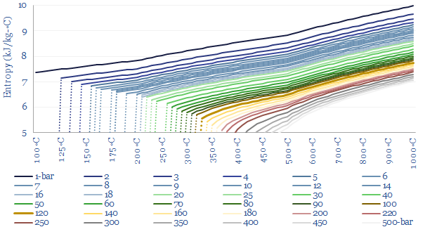
Enthalpy versus entropy. These two steams in our example above, despite having the same enthalpy, have different entropies. Steam at 280◦C and 10-bar has an entropy level of 7.0 kJ/kg-K. Steam at 460◦C and 250-bar has an entropy level of 5.7 kJ/kg-K (chart below). The entropy of a system does not change unless heat flows in or out of the system. The concept of entropy is explained in more detail in our overview of thermodynamics.
Entropy of steam versus temperature and pressure
What this means in practice is that compressing a 280◦C gas stream from 10-bar to 250-bar — isentropically, i.e., without letting any heat transfer take place into or out of the steam — would absorb about 1.2 GJ/ton of compression work, and this would naturally tend to heat the steam up to about 850◦C. You can read this off the chart above by moving ‘left to right’ along the same horizontal line. This is simply how the gas laws go for steam. You could then extract useful heat from the steam as it cools back down to 460◦C, lowering both its enthalpy and its entropy. The enthalpy extracted would be, you guessed it, 1.2 GJ/ton. And if you later wanted to ‘get back’ to the starting point of 10-bar and 280◦C then ultimately you would need to flow heat energy into the system, to raise the entropy back to its original value. These values are simply read from the steam data tables compiled in this data-file.
In order to avoid violating the laws of thermodynamics, it is usually necessary to model compressions and expansions as being isentropic. Assume that heat energy cannot flow in or out of the system during the compression or expansion process, and thus that entropy remains constant. This is why we need steam tables, like the ones aggregated in this data-file, to show how actual energy flows will behave and quantify the energy needed to produce steam. The data-file captures density, volume, enthalpy, internal energy, PV energy and entropy at 100 x 40 different temperatures and pressures.
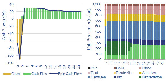
Hydrogen peroxide production costs run at $1,000/Tpa, to generate a 10% IRR at a greenfield production facility, with c$2,000/Tpa capex costs. Today’s market is 5MTpa, worth c$5bn pa. CO2 intensity runs to 3 kg of CO2 per kg of H2O2. But lower-carbon hydrogen could be transformational for clean chemicals?
Hydrogen peroxide is a 5MTpa and $5bn pa commodity chemical market. It is an oxidizing agent, used in producing paper, detergents and in water treatment. And increasingly in producing materials that matter for the energy transition, such as propylene oxide for polyurethaneinsulation/EVs and for etching semiconductors.
Hydrogen peroxide production costs? This data-file estimates the economic costs of producing hydrogen peroxide, at $1,000/ton per ton of 100%-pure H2O2. An important definitional point is that H2O2 is often transported at 30-70% concentration, then later diluted for end use at 3-8% concentration. Clearly, the more you dilute the product, the more you dilute the price. But our numbers are per (hypothetical) ton of pure H2O2.
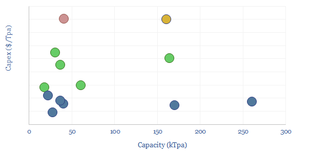
Capex costs of hydrogen peroxide plants also vary by technology, product concentration and product purity. Please see the data-file for further details. But our base case is around $2,000/Tpa of capex costs for a new, greenfield hydrogen peroxide plant. High purity hydrogen peroxide for the semiconductor industry costs more.
Capex costs of hydrogen peroxide production facilities
How is hydrogen peroxide produced? The dominant method is anthraquinone auto-oxidation. The key input is hydrogen, which reduces anthraquinone. The reduced anthraquinone can later be oxidized, in the presence of air, forming both H2O2 and H2O, and regenerating the anthraquinone. The process uses a palladium catalyst. It is exothermic, so heating inputs are low.
How much hydrogen is used up in making hydrogen peroxide? The key challenge is minimizing over-consumption of hydrogen (or in other words, maximizing hydrogen conversion and selectivity). Our estimates into hydrogen consumption of hydrogen peroxide production are tabulated in the data-file.
The CO2 intensity of hydrogen peroxide production is 3 tons/ton, as our base case estimate, for today’s production process. The largest contributor is the embedded CO2 of hydrogen, which also comprises one-third of total hydrogen peroxide production costs.
Could clean hydrogen be a game-changer? What if IRA incentives allow hydrogen peroxide plants to source cheaper hydrogen? Each $0.1/kg reduction in the input hydrogen price raises cash flow by 8% and IRRs/ROCEs by a full percentage point (1pp). Our best single note on booming blue hydrogen value chains is linked here.
Low carbon hydrogen can realistically reduce the CO2 intensity of hydrogen peroxide from 3 kg/kg, to below 0.5 kg/kg. Further downstream, this can reduce the total CO2 intensity of propylene oxide production from 2-3 kg/kg to 1 kg/kg. Further downstream, propylene oxide can react with CO2 in a molar ratio of 1:1 (forming polyether polycarbonates) or 2:1 (forming polycarbonate polyols), and switching in low-carbon hydrogen can make these overall value chains close to carbon neutral for the polyether polycarbons, and substantially lower carbon for downstream polyurethanes.
Leading hydrogen peroxide producers, such as Solvay, Evonik and Arkema, may thus benefit from low carbon hydrogen? Some recent notes on each company are in the data-file. Evonik purchased PeroxyChem for $640M in 2020, consolidating the global hydrogen peroxide market. In June-2023, Solvay said it would develop Europe’s first hub for the production of “green hydrogen peroxide” by mid-2026, with a 9.5MW dedicated PV installation, yielding 756Tpa of green hydrogen, to reduce Solvay’s total CO2 footprint at its Rosignano plant by 15%.
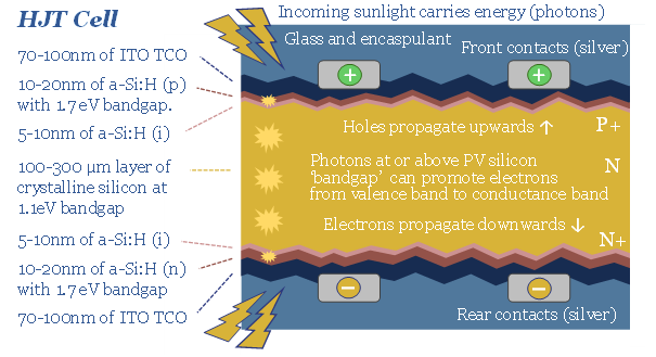
HJT solar modules are accelerating, as they are highly efficient, and easier to manufacture. But HJT could also be a kingmaker for Indium metal, which is used in transparent and conductive thin films (ITO). Our forecasts see primary Indium use rising 4x by 2050. Indium is 100x rarer than Rare Earth metals. It could be a bottleneck. This 16-page note expores the costs and benefits of using ITO in HJTs, and who benefits as solar cells evolve?
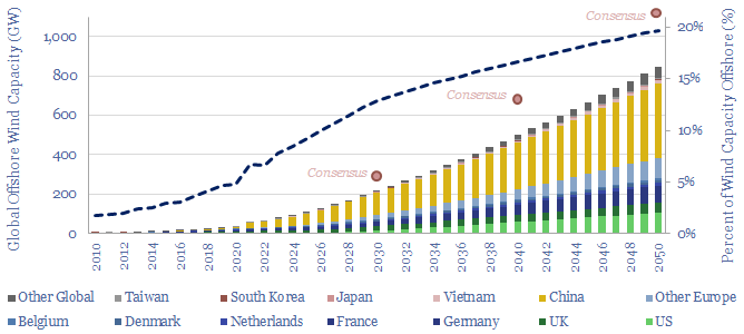
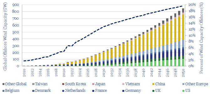
Global offshore wind capacity stood at 60GW at the end of 2022, rising at 8GW pa in the past half decade, comprising 7% of all global wind capacity, and led by China, the UK and Germany. Our forecasts see 220GW of global offshore wind capacity by 2030 and 850GW by 2050, which in turn requires a 15x expansion of this market.
Installed global offshore wind capacity stood at 60GW at the end of 2022, representing 7% of all global wind capacity installed to-date, based on helpful data from GWEC.
The largest offshore wind capacity bases among different countries are in China (31GW, meaning that 9% of China’s total wind capacity was offshore), the UK (14GW, 50% of total capacity is offshore) and Germany (8GW, 12% of total capacity is offshore).
Global offshore wind capacity forecasts by 2030 that have crossed our desk range from 200-400GW, and our own estimate is towards the lower end, at 220GW, which would be 13% of all global wind capacity.
Global offshore wind capacity forecasts by 2050 that have crossed our desk range from 600-2,000GW, and our own estimate is also towards the lower end, at 850GW, which would be 20% of all global wind capacity.
Please download the data-file to explore offshore wind capacity by country, and how the market might evolve. Our numbers are top-down estimates, approximations that seem reasonable to us, based on the size of the grid in each region, the share that can realistically come from wind, and the percent of wind that can realistically come from offshore, linking between various TSE energy market models.
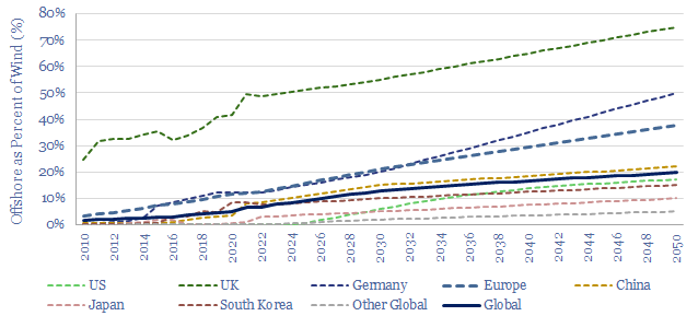
Share of Total Installed Wind Capacity that is Offshore by Country by Year with Forecasts to 2050
Mathematically, if total installed wind capacity rises by 5x by 2050, and offshore’s share of that capacity rises 3x (from 7% to 20%) then offshore capacity is rising by about 15x, which is one of the larger ramp-ups required in our roadmap to net zero.
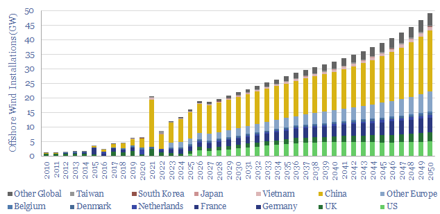
Offshore wind installations averaged 8GW per year in 2018-22, and must rise by 5x to 40GW per year in the 2040s (chart below).
Offshore Wind Installations by Country by Year in GW from 2010 to 2050
Offshore wind capex requirements? At an average cost of $4,000-5,000/kW, this would require about $160-200 bn per year of capex, for comparison with other market sizes. For further details on our capex build-up, please see our offshore wind cost model.
Offshore wind generation in TWH? At an average capacity factor of 40% on installed capacity, the numbers in this data-file would translate into about 3,000 TWH of useful offshore wind energy, or 3% of the global total useful energy in our global energy demand models.
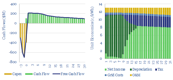
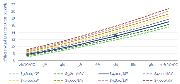
This model estimates the levelized cost of offshore wind at 13c/kWh, to generate a 7% IRR off of capex costs of $4,000/kW and a utilization factor of 40-45%. Each $400/kW on capex adds 1c/kWh and each 1% on WACC adds 1.3 c/kWh to offshore wind levelized costs.
The levelized costs of offshore wind are built up in this economic model, and a flat price of 13c/kWh is needed, over a 25-30 year project life, in order to generate a 7% IRR.
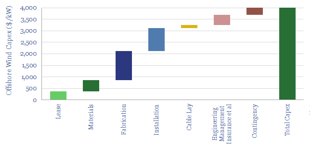
Offshore wind capex will tend to average $4,000 per kW according to our build-up
Operating costs of wind turbines are aggregated in our data-file here. Decline curves of wind turbines are aggregated in our data-file here. Our estimate of grid connection charges is based on tracking past projects and the need for synthetic inertia and reactive power compensation. Decision-makers are welcome to reflect or ignore these costs, but we recommend understanding them and reflecting them.
Levelized costs of offshore wind are most dependent upon WACCs, as effectively all of the costs are capex costs, incurred up front, unlike other power generation sources. A rule of thumb is that each 1% variation in WACC impacts levelized cost by 1.3 c/kWh and each $400/kW on the capex impacts levelized cost by 1c/kWh. Although for more detailed numbers, these two variables are interdependent (sensitivity chart below).
Sensitivity of offshore wind costs to capex costs and WACCs
What is the levelized cost of offshore wind? Our 13c/kWh estimate is a flat estimate over 25-30 years. I.e., it means that the weighted average sales price of electricity must run at 13c/kWh in order to generate a 7% IRR. We would note that some other commentators have published levelized costs using quite different financial assumptions…
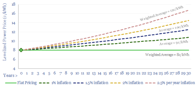
Some other commentators have WACCs in the range of 3-5% (the Fed Funds Rate is above 5% in 2023). Others publish numbers on a ‘real’ basis, which means that the price in Year 1 escalates over time, e.g., with inflation. So for example, what is quoted as an 8c/kWh ‘real levelized cost’ really means 10c/kWh over the life of the project and 14c/kWh by the end of the project (chart below). To be clear, our numbers are nominal numbers, and do not juice the IRR by assuming an annual price escalation.
Levelized costs can be defined in nominal terms or in real terms
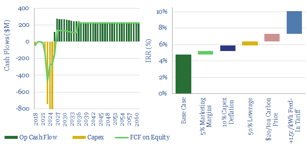
A detailed case study is also presented in the data-file, covering the 816MW Empire Wind project, off New York, constructing c80 x c10 MW wind turbines, each as tall as the Chrysler building. Base case IRRs would be in single digits. The model explores how hypothetical initiatives might uplift the returns, including power marketing, continued cost-deflation, leverage, carbon prices and feed-in tariffs (chart below).
Empire Wind Uplifts 5 percent IRR to 10 percent IRR via incentives leverage and tariffs
Please download the data-file to stress test the economics of offshore wind projects, and see how levelized costs vary with capex, opex, utilization rates, taxes and other costs. For comparison, our economic model for onshore wind projects is linked here.
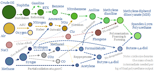
Polyurethanes are elastic polymers, used for insulation, electric vehicles, electronics and apparel. This $75bn pa market expands 3x by 2050. But could energy transition double historically challenging margins, by freeing up feedstock supplies? This 13-page note builds a full mass balance for the 20+ stage polyurethane value chain and screens 20 listed companies.
Cookies?
This website uses necessary cookies. Our cookies are simply to improve your experience. We do not undertake any advertising or targeting via our cookies. By clicking 'accept' or continuing to use the website, you consent to our use of cookies.AcceptRead More
Privacy & Cookies Policy
Privacy Overview
This website uses cookies to improve your experience while you navigate through the website. Out of these, the cookies that are categorized as necessary are stored on your browser as they are essential for the working of basic functionalities of the website. We also use third-party cookies that help us analyze and understand how you use this website. These cookies will be stored in your browser only with your consent. You also have the option to opt-out of these cookies. But opting out of some of these cookies may affect your browsing experience.
Necessary cookies are absolutely essential for the website to function properly. This category only includes cookies that ensures basic functionalities and security features of the website. These cookies do not store any personal information.
Any cookies that may not be particularly necessary for the website to function and is used specifically to collect user personal data via analytics, ads, other embedded contents are termed as non-necessary cookies. It is mandatory to procure user consent prior to running these cookies on your website.