Downloads Insights- Thunder Said Energy

Demand shifting: electrical flexibility by industry?

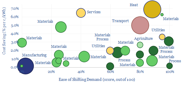
Demand shifting is the process of flexing electrical loads in a power grid, in order to smooth out volatility. Especially short to medium-duration volatility associated with wind and solar. This database scores technical potential and economical potential of different electricity-consuming processes to shift demand, across materials, manufacturing, industrial heat, transportation, utilities, residential HVAC and commercial loads.

Renewable output is volatile. Solar generation is volatile. Wind generation is volatile. The volatility spans from second-to-second volatility, through to minute-by-minute, hour-by-hour, day-by-day, season-by-season and even year-by-year.

Demand shifting is an excellent solution. It may be easy. It may cost nothing. It may not incur any energy penalties. Unlike batteries and hydrogen. And we think that ultimately 20-30% of the power grid may ultimately able be able to shift demand in some way.

To put it more bluntly, if your investment thesis for grid-scale batteries and green hydrogen is that electrolysers will be able to mop up “free power” at times when excess renewables “have nowhere else to do”, then here is a catalogue of 25+ other commercial and industrial that can literally start printing money first, simply using smart logic and power electronics, but without having to make any major new capital investments.

What is demand shifting? Demand shifting might involve turning an electrical load off when renewables are not generating, and turning it back on when renewables are generating. Or as a less extreme example, demand shifting might involve turning an electrical load down when renewables are not generating, and turning it back up when renewables are generating.

Electric vehicle chargers can slow their current flow minute-by-minute, or time non-critical charging activities for off peak times (note here, model here).

In residential heat, likewise, imagine a house that has both a gas-fired boiler and/or a heat pump and/or a resistive electrical heater in its well-insulated hot water tank. It is trivial to shift loads by a few minutes-hours, or switch between gas heating and electrical heating depending on prevailing prices. Especially with help from smart energy systems or predictive AIs.

In utilities, a nice example is the production of water by reverse osmosis, which yields 35bn tons of desalinated water each year, absorbing 250 TWH of electricity, as pumps force water molecules – but not salt ions – across a semi-permeable membrane, using about 3-4 kWh/m3 of pumping energy. Pumps can easily ramp up and shut down, and each 1c/kWh saved would decrease the cost of desalinated water by around 3.5% (membrane note here, osmosis model here). Similar examples include pipelines and utility pumps.

In the tech industry, the internet uses 1% of all global energy and 2% of all global electricity, of which one-third is data-centers (note here). But around 40% of data center loads can be shifted, of which two-thirds is temporal shifting and one-third is routing process loads to a data center at a different geographic location (more here).

In materials, there is great opportunity for demand shifting, because EBIT margins are usually around 20% and electricity is often c10% of total costs. If demand shifting save around 1c/kWh, or around 1pp of electricity cost, this is tantamount to a 5% uplift on EBIT, and by extension, a 5pp uplift on ROCE.

Whether materials can demand shift is highly dependent on the material production process, which itself can get quite complex. A “simple” pulp and paper plant has 18 separate stages, from de-barking (easy to flex) to pressing and drying (the process may need to be precisely controlled in order to make specialty grades of paper).

Across the materials industry, this data-file considers cement plants, industrial gas production, electric arc furnaces, aluminium, chlor-alkali, polymers, paper, silicon, sulphur, glass, hydrofluoric acid, small-scale hydrogen and hydrogen cyanide.

A best to worst ranking depends on the technical potential and economic potential. An electric arc furnace for steel recycling might typically have a low utilization as it is constrained by the ability to source scrap. A cement plant might use 110kWh/ton of electricity, of which 100kWh/ton is a non-time-critical comminnution circuit, grinding input rocks and output clinker into talcum powder. It may be easy to flex these loads and offer large savings. Conversely, you probably do not want to tinker with the process flows in a 1,100ºC process moving toxic gases when making Hydrogen Cyanide, or risk damaging semiconductors as pure silicon boules are crystallized out at 25 mm per hour in the Czochralski process.

Mining processes perhaps screen best of all? Processes such as communition, flotation, heap leaching and electrowinning screen as some of the most flexible processes in our entire data-file. And indeed, the Super-Majors of energy transition may include Super-Miners, as metals and materials demand booms.

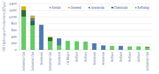
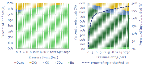
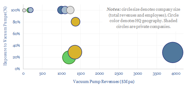
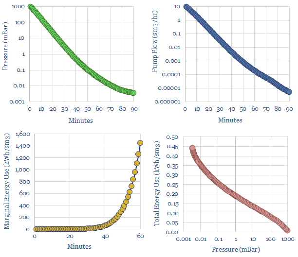
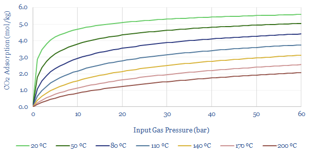
In industrial gases, there is also a fascinating shift underway, where pressuring swing adsorption (using compressors and vacuum pumps, note here) is much more flexible than cryogenic plants that take days to cool down (note here).

Manufacturing operations may generally find it harder to demand shift. Consider that a modern auto plant might assemble a car by moving each vehicle along a production line with c1,000 x 1-minute discrete stages, in a continous process, where pausing any one stage effectively halts the entire line; and a full scale auto plant employs 1,000-3,000 people, whose sudden idling would be very expensive for the auto-maker (model here).

This data-file will serve as our reference file for which processes can shift demand and use demand shifting to integrate more renewables. We will continue building the data-file out over time.

European gas and power model: natural gas supply-demand?

This data-file is our European gas supply demand model. Balances are assessed in European gas and power markets from 1990 to 2030, reflecting all of our research into the energy transition. 2023-24 gas markets will look better-supplied than they truly are. We think Europe will need to source over 15bcfd of LNG through 2030. A dozen key input variables can be stress-tested in the data-file.

Europe’s gas demand averaged 45bcfd in the decade from 2012 to 2021, of which c30% was consumed in industry, c30% in residential heating, c10% in commercial heating, c25% in electricity generation, and smaller quantities in T&D and transportation (chart below). Gas demand is disaggregated across a dozen different industries in the data-file.

European gas demand fell back below 40bcfd in 2022. We think that one half of the decline can be attributed to a particularly warm winter, and will naturally come back with more normal winter weather. And total demand will run sideways through 2030.

Gas demand in the European power market is actually seen rising from 11bcfd in 2021 to 13bcfd by 2030, as the electrification of heat and vehicles raise overall demand, while decarbonization ambitions are also likely to phase down 2.5x more CO2 intensive coal (chart below).

Europe’s indigenous gas supply looks increasingly pathetic. We will likely fall below 7bcfd of domestic gas production in 2023, down from a peak of 24bcfd, 20-years ago. Even amidst the supply disruptions of 2022, there is no sign yet that Europe is seriously considering long term supply growth. Although there is vast potential in European shale.

Europe has doubled its reliance on imports over the past 20-30 years, rising from a 40-45% share of final demand in 1990-2004, to an 80-85% share in 2021-25. Thank god for Norway, which is also the cleanest and lowest carbon gas in the world.

Recently, Russian supplies have collapsed, while our outlook sees a large pull on global LNG through 2030. We think this will support LNG prices.

Although in 2023-24, European gas markets may look better supplied than they really are, due to excess inventories, that were built up as an insurance policy in 2022. This is temporary.

The data file also contains granular data, decomposing gas demand across 8 major categories, plus 13 industrial segments, going back to 1990 (albeit some of the latest data-points are lagged); as well as 15 different supply sources, with monthly data going back a decade (chart below).

All models are wrong, but some models are useful. Hence variables that can be flexed in the model, for stress-testing purposes, include the growth rates of renewables (wind and solar), the rise of electric vehicles, the rise of heat pumps, the phase out of coal and nuclear, industrial activity, efficiency gains, LNG and hydrogen.

Please download the model to run your own scenarios. Our numbers have changed since the publication of our latest outlook for European natural gas, but if anything, we see the same trends playing out even moreso.

US hydrogen production: by facility and by company?

10MTpa of hydrogen is produced in the US, of which 40% is sold by industrial gas companies, 20-25% is generated on site at refineries, 20% at ammonia plants and 15-20% in chemicals/methanol. This datafile breaks down US hydrogen production by facility. Owners of existing steam methane reforming units may readily be able to capture CO2 and benefit from CO2 disposal credits under the US Inflation Reduction Act?

Methodology. As far as we are aware, there is no publicly available database of US hydrogen production by facility. However, we have cleaned up facility by facility data from EPA FLIGHT, which show CO2 emissions by facility, and then used some rules of thumb to estimate hydrogen production. For example, our methane reforming model estimates 9 tons of CO2 are emitted per ton of hydrogen. Our ammonia models estimate 0.2 tons of hydrogen per ton of ammonia, and 2.5 tons of CO2 per ton of ammonia. We then spent a day scrubbing the data and comparing our numbers with publicly available information from different companies. Our conclusions follow.

The US produces 10MTpa of hydrogen each year, of which c40% is merchant hydrogen sold by industrial gas companies, 20-25% is generated on site at refineries, c20% is at ammonia plants and c15-20% is at methanol/chemicals facilities (chart below). The solid bars are fully disaggregated, facility by facility, in the database. We also added increments to reflect facilities that do not report to FLIGHT, catalytic reforming units at refineries, and other chemical generation of hydrogen, especially methanol plants.

Two states on the US Gulf Coast, Texas and Louisiana, dominate the mix, with around 45% of total US hydrogen production, and c65% of total merchant hydrogen production.

Similarly, three industrial gas giants, Air Products, Linde and Air Liquide dominate the industry, producing well over 90% of the US’s merchant hydrogen, and c30-40% of all US hydrogen.

Also among the US’s major hydrogen producers are ammonia companies and oil refiners. Refineries currently consume 70-80% of all merchant hydrogen sales from industrial gas companies in the US. Some large and famous refiners purchase effectively all of their refinery hydrogen from third parties. For example, ExxonMobil has a long-standing partnership with Air Products (highlighted by Air Products here).

But other refiners operate their own SMRs and produce their own hydrogen on site. One Oil Major and two refiners stand out, with over 300kTpa of annual hydrogen production (all of the different companies are covered in the database and in our broader US refinery database).

Where this gets interesting is that the US Inflation Reduction Act (45Q) offers $85/ton cash incentives to companies that can capture and sequester CO2. In our view, capturing CO2 from existing Steam Methane Reformers is technically ready, relatively simple (compared to other CCS opportunities with high energy penalties and amine degradation issues), and can earn 20% IRRs when we model the costs and a share of 45Q revenues (chart below). The company that owns the reformer is the one that will be able to benefit from the 45Q credits. So we wonder which industrial gas companies, refiners and chemicals plants from the data build-up overleaf will grasp this opportunity.

Please download the database for our estimated breakdowns of US hydrogen production, facility by facility and operator by operator.

Omniscience: how will AI reshape the energy transition?

AI will be a game-changer for global energy efficiency. It will likely save 10x more energy than it consumes directly, closing ‘thermodynamic gaps’ where 80-90% of all primary energy is wasted today. Leading corporations will harness AI to lower their costs and accelerate decarbonization. This 19-page note explores the opportunities.

Lithium ion batteries: energy density?

Today’s lithium ion batteries have an energy density of 200-300 Wh/kg. I.e., they contain 4kg of material per kWh of energy storage. Technology gains can see lithium ion batteries’ energy densities doubling to 500Wh/kg in the 2030s, trebling to 750 Wh/kg by the 2040s, and the best possible energy densities are around 1,250 Wh/kg. This is still 90% below hydrocarbons, at 12,000 Wh/kg. Numbers and underlying assumptions are broken down in this data-file.

The energy stored in a battery can be calculated by thinking about the active ions. Active ions are intercalated at the anode when the battery is charged. They surrender electrons to an external circuit. Then these ions diffuse across the electrolyte. Finally, they intercalate at the cathode, where electrons are re-accepted. Thus the energy stored (in Joules) can be calculated by multiplying Faraday’s Constant (in Coulombs per mol) by the cell voltage (in Volts) and the number of mols of ions making this journey from anode to cathode (in mols).

Today’s lithium ion batteries have an energy density of 200-300 Wh/kg. In other words, there is 4kg of material per kWh of energy storage. Of this material build-up, 2 kg is in the cathode, 1 kg is in the anode, 0.6 kg in the current collectors, 0.3 kg in the electrolyte and 0.1 kg in the balance. Different chemistries are assessed in our data-file here.

The maximum energy density of a lithium ion battery can be calculated by increasing the voltage and decreasing the weights of all of the other components. So how much can the energy density of lithium ion batteries improve?

For example, today’s graphite anodes only intercalate 1 lithium ion for every 6 graphite atoms, which weigh 12 g/mol, yielding a charge density of 372 mAh/gram. Silicon anodes weigh more (28g/mol), but they can intercalate 15 lithium ions per 4 silicon atoms, yielding a charge density of 2,577 mAh/gram. (Satisfyingly, these numbers are calculated from first principles in the data-file). So this is an avenue being explored by Amprius, Sila, Enovix. Even denser, could be solid state batteries.

We think the best lithium ion batteries could ultimately reach 1,250 Wh/kg energy densities, although this includes some heroic assumptions and technology gains. It includes a 50% increase in cell voltage, eliminating the anode, eliminating all other excess materials, doubling the charge density of the cathode, thrifting out 90% of the electrolyte and 50% of the current collectors and separators. You can stress test all of these numbers in the data-file.

The biggest uncertainty, in our view, is over cell voltages. Today’s lithium ion batteries run at an average mid-point of 3.6V. Energy density is a direct linear function of voltage. But excess voltages will degrade the battery. For example, 5.9V is the standard potential for decomposition LiF into Li metal and fluorine gas (!).

Could sodium ion batteries have higher energy density? Basic chemistry of the periodic table makes it quite unlikely that any other metal ion could ferry ‘holes’ across an electrochemical cell with the same energy density as lithium. Lithium ions carry a charge of +1 and have a molar mass of 6.94 g/mol. Sodium ions carry a charge of +1 and have a molar mass of 22.9 g/mol.

The energy densities of lithium ion batteries are, in our view, unlikely to surpass 1,250 Wh/kg, on realistic technology pathways, simply based on electrochemistry and simple molar masses, which are broken down in this data-file. This can be compared with the energy density of hydrocarbons and as calculated from bond enthalpies.

Even 200-300Wh/kg energy density of lithium ion batteries justifies the electrification of light passenger vehicles, as electric motors are 2-6x more efficient than combustion engines. But we still see high-density hydrocarbons retaining a major role in aviation, long-distance trucking and shipping. These numbers underpin some of our key vehicle conclusions, hydrocarbon conclusions and battery conclusions amidst the energy transition.

Industrial gas separation: swing producers?

Swing Adsorption separates gases, based on their differential loading onto zeolite adsorbents at varying pressures. The first PSA plant goes back to 1966. Today, tens of thousands of PSA plants purify hydrogen, biogas, polymers, nitrogen/oxygen and possibly in the future, can capture CO2? This 16-page note explores the technology, costs, challenges, companies.

Vacuum pumps: company screen?

The global market for vacuum pumps is worth $15bn per year, with growing importance for making semiconductors, solar panels and AI chips. This data-file reviews ten leading companies in vacuum pumps, including one European-listed capital goods leader, a European pure-play and a Japanese-listed pure-play.

The vacuum pump market is worth $15bn per year, and some sources imply that over half of the market now comprises semiconductor applications, such as the vacuum chambers used for vapor deposition and sputtering, when manufacturing AI chips and solar cells.

Other applications, back in the traditional industrial landscape, use vacuum pumps. Ranging from the food manufacturing industry (one company website that we reviewed comprehensively lists how their technology is used in making cheese), through to gas separations via swing adsorption, membranes or petrochemicals.

Many processes in the semiconductors are remarkable because they use vacuum chambers to prevent contamination from, and reaction with, atmospheric air, when depositing thin film layers of 5-250 nm. If normal pressure is 1 bar, some of these processes can occur at 0.001 mBar, i.e., 1 millionth of an atmosphere.

Evacuating a vacuum chamber down to 0.1-0.001 mBar can take 90+ minutes, while the pump continues working, pumping out ever smaller quantities of air, which equates to an exponentially rising energy consumption per unit of sm3 of air that is pumped. As a rule of thumb, we think that reaching 0.1-0.01 mBar will require 0.3-0.5 kWh of electricity per m3 of volume in the vacuum chamber (charts below).

Atlas Copco is the industry leader in vacuum pumps. Its market share, and recent acquisitions are explored in the data-file. But total group operating margins were 21% in 2022 and ROCE was 29%. Vacuum pumps comprise 28% of the company’s revenues. In its vacuum pump business, Atlas Copco’s 2022 orders were 65% electronics and semiconductors, 21% chemicals/process industries including the food packaging industry and 12% general manufacturing. More via the Atlas Copco website. But this is interesting, as Atlas Copco has screened well in other areas of TSE research, such as in compressors, increasingly important for industrial gases and CCS value chains.

Other leading companies in vacuum pumps? Listed pure-plays in both Germany and Japan also feature in the data-file. Plus industrial conglomerates in the US, Europe and Japan, with varying concentration.

There are some interesting data-points in the commentary about who leads in supplying vacuum pumps to the semiconductor industry.

Electric vehicles: breaking the ICE?

Electric vehicles are a world-changing technology, 2-6x more efficient than ICEs, but how quickly will they ramp up to re-shape global oil demand? This 14-page note finds surprising ‘stickiness’. Even as EV sales explode to 200M units by 2050 (2x all-time peak ICE sales), the global ICE fleet may only fall by 40%. Will LT oil demand surprise to the upside or downside?

Adiabatic flame temperature: hydrogen, methane and oil products?

This data-file is a simple model calculating adiabatic flame temperatures from first principles. At an idealized, 100% stoichiometric ratio, the adiabatic flame temperature for natural gas is 1,960ºC, hydrogen burns 300ºC hotter at 2,250ºC and oil products burn somewhere in between, at around 2,150ºC. However, the calculations also show why hydrogen cannot always be dropped into an existing turbine or heat engine that was previously designed to run on other hydrocarbons.

What is adiabatic flame temperature?

Adiabatic flame temperature denotes the maximum theoretical temperature that can be reached by a mixture of gases during combustion, if precisely all of the enthalpy of combustion (in kJ/mol) is transferred directly into those gases.

Hence adiabatic flame temperature can easily be calculated from first principles, as a function of (a) the different input gases; (b) the resultant exhaust gases; (c) the masses of those gases (in kg); and (d) the specific heat capacity of each gas (Cp), which is the amount of energy needed to raise its temperature by 1-degree (in kJ/kg-K).

A 100% equivalence ratio denotes the condition where 100% of a fuel combusts perfectly and reacts with 100% of the oxygen in the input mixture. This 100% stoichiometry will naturally maximize the temperature of the resultant flame, because no heat is dissipated unnecessarily in heating up superfluous oxygen.

The data-file shows that at an idealized, 100% stoichiometric ratio, the adiabatic flame temperature for natural gas is around 1,960ºC, hydrogen burns 300ºC hotter at 2,250ºC and oil products burn somewhere in between, at around 2,150ºC. Satisfyingly, these bottom-up calculations match the widely quoted adiabatic flame temperatures shown in online resources such as Wikipedia.

Why does adiabatic flame temperature matter in industry?

Very hot process temperatures are needed for producing many metals, materials and in some hydrogen reforming reactors.

For example, a blast furnace can reach 1,100-1,600ºC. Cement plants decompose CaCO3 into clinker at 1,400-1,500ºC. Mined lithium ores are roasted at 1,100ºC to change the crystal structures of spodumenes. In semiconductor, mono-crystalline polysilicon for chips and solar panels is grown via the Czochralksi method at 1,425ºC; while the SiC used in cutting edge EV power-MOFSETs is grown at 2,000ºC in the Lely process. The heating-melting temperatures of different solids are compared here.

Reaching these very hot process temperatures requires a materially hotter flame temperature. You clearly cannot heat a process to 1,500ºC with a 1,000ºC flame.

Real world flame temperatures will tend to be lower than the adiabatic flame temperatures at 100% equivalent ratios, quoted above for methane, hydrogen and oil products.

Real world processes are not adiabatic. An adiabatic process is one where no energy is transferred in or out of the system. But in the real world, the entire point of generating heat is to transfer it out of the system and do some useful work, for example by driving a turbine or supplying energy into an endothermic chemical reaction.

Some combustion enthalpy will always be lost to heating the surrounding reactor/plant, reagents, and leaked into the surroundings.

We used Cp as our specific heat capacity, which reflects the fact that some of the combustion enthalpy is expended in expanding the gases rather than just heating them up. Cp values rise with temperature. It gets incrementally harder to heat up hot gases (chart below).

Finally, in the real world, it is not recommended to fire a combustion reactor too close to 100% stoichiometry, otherwise the result may be incomplete combustion forming soots, carbon monoxide and nasty NOXs.

So in practice, if you are going to run a reactor with 1.5-2x the stoichiometric minimum oxygen content, as a margin of safety against incomplete combustion, in a real-world plant with heat losses, it can be challenging to achieve >1,000ºC process temperatures by burning fuels like natural gas, oil products or coal in an atmosphere of air (chart below).

Achieving very high process temperatures often requires enriching fossil-fired combustion processes with additional oxygen beyond the 21% molar fraction found in air.

This need for super-high process temperatures is a key driver behind global industry’s 400MTpa oxygen demand, per our note below.

Industrial gases: out of thin air?

Flame temperature: can you blend hydrogen into existing heat engines?

The analysis of adiabatic flame temperature also shows why hydrogen cannot always be blended into pre-existing turbines or engines that were intended to be run on some different hydrocarbon, without some important engineering considerations.

For example, consider a gas turbine that has been designed to burn a mixture of 4-6% methane and 94-96% air, which equates to a 67-150% stoichiometric excess of oxygen, yields a maximum flame temperature around 900-1,250ºC, and an exhaust gas with around 4-6% CO2 concentration (calculations in the data-file).

Well, replace the 6% methane input with a 6% hydrogen input, and the adiabatic flame temperature only reaches about 450ºC. The reason is that each mol of hydrogen only releases one-third of the combustion enthalpy as each mol of methane (numbers in the file). All else equal, this lower temperature would detract over 20% from the energy efficiency of a typical Brayton Cycle. Oh dear.

You could increase the temperature back to the original 1,250ºC target by mixing a 3x higher blend of hydrogen into the input gases. But now there are questions about whether the inlets can flow these higher volumes of fuel gas, whether the gases will mix evenly; or conversely, will there be localized hotspots with annoying consequences like melting your burner tips, or other parts of your plant.

Likewise an engine burning liquid hydrocarbons might only be spraying a mist of 0.5-1% oil products by volume into a combustion cylinder before ignition at 700-1,400ºC, according to these adiabatic flame temperature calculations.

If hydrogen is used as a combustion fuel, it will result in materially higher volumetric flow rates to generate the same temperatures as natural gas or liquid hydrocarbons.

When burned at its optical stoichiometric ratio, hydrogen will also yield 300ºC higher temperatures than burning methane. This can be a blessing in terms of thermodynamic efficiency. But conversely, the limit on pre-existing gas turbines is not the ability to generate high flame temperatures. It is the ability to withstand them! For example, via the temperature resiliency of cutting-edge super-alloys. And this is a key reason why gas turbines tend to flow excess air as coolant or re-circulate exhaust gases.

To control a process temperature, while blending in varying molar fractions of hydrogen, requires careful calculation. More hydrogen means more demand for engineering services, in our view.

Pressure swing adsorption: energy economics?

Pressure swing adsorption purifies gases according to their differing tendencies to adsorb onto adsorbents under pressure. Pressure swing adsorption costs <$0.1/kg when separating pure hydrogen from the output of reforming reactors, and maybe $2-3/mcf when separating bio-methane from biogas. The cost breakdowns in this data-file include capex, opex, maintenance, zeolite replacement, compression power and CO2 costs.

Pressure swing adsorption compresses a mixture of gases against a solid bed of adsorbents. Different gases ‘adsorb’ onto the surface of this material at different rates, defined by their enthalpy of adsorption (exothermic), partial pressures and temperatures.

This effect is called differential loading. By pulsing gas into a chamber at high pressure, commonly 10-30 bar, gases with lower affinity to the adsorbent can be concentrated in the productate stream, while gas with higher affinity to the adsorbent remain in the chamber until the low affinity gases have been purged and the adsorbent is depressurized.

The physics can be complex, but in the data-file, we have applied some simple equations for multi-component Langmuir isotherms, especially for separating hydrogen out of reforming tail gases, and for CH4/CO2 separations in biogas. We have also played around with some more complex models such as Sips and Toth models (chart below).

But mainly, the data-file is not intended to be overly precise in capturing the physics of pressure swing adsorption, for which we recommend chemical engineering software.

Our goal is to aggregate data-points into the capex, opex, costs, energy use, purity and recovery of PSA processes, as used in present and future industrial applications.

Pressure swing adsorption costs <$0.1/kg when separating hydrogen out of tail gas from the water gas shift reaction of a steam methane reformer, in producing grey or blue hydrogen; and costs $2-3/mcf when separating biomethane out of biogas.

For example, the data imply that the average PSA gas separation will cost $70/Tpa in capex, yield 98% pure product, with 85% recovery from input feeds, and the energy use will average 400 kWh/ton as a mid-point (although it can range from 20-2,000 kWh/ton). The energy costs of pressure swing adsorption are going to depend on pressures used and the energy demands of gas compression.

Please download the data-file to stress-test your own economic assumptions, and for the breakdown of pressure swing adsorption costs. Other techniques for gas separations include amine separations, membrane separations and cryogenic separations.

What is adiabatic flame temperature?

Why does adiabatic flame temperature matter in industry?

Flame temperature: can you blend hydrogen into existing heat engines?

Cookies?