Metals
-
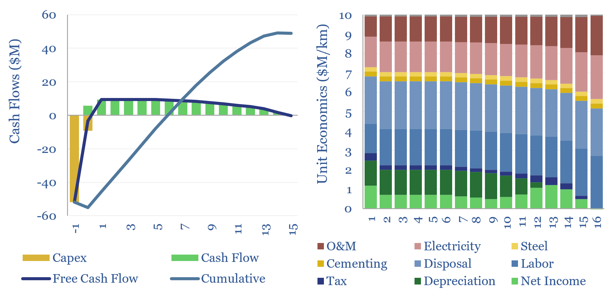
Tunnel boring: the economics?

The global market for tunnel boring machines has been estimated at $7.5bn pa. But what are the costs of tunnel boring? This data-file models tunnel boring economics, estimated at $10M/km for civil infrastructure projects today, $30M/km for deep mine shafts, but will cheap solar and autonomous robots deflate costs?
-
Global iron ore production by company over time?

Iron ore is the sixth most produced commodity in the world, at 2.7GTpa. This data file breaks down global iron ore production by company over time. Since 2019, average realizations for the largest producers have risen at 1.6% pa, while costs have risen at 5% pa. What outlook from here?
-
Copper companies: a screen of leading producers?
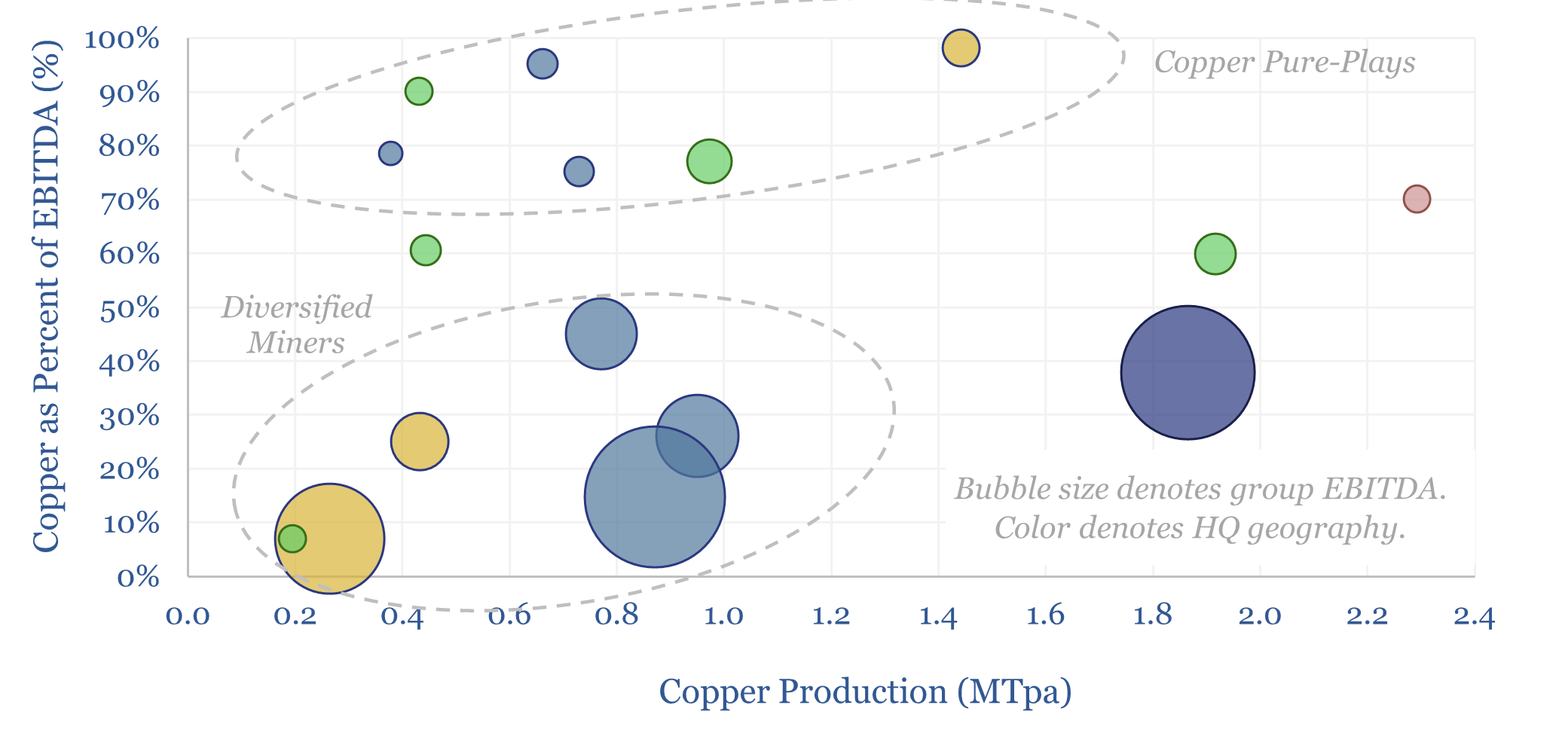
This data-file is a screen of the world’s largest copper companies, across c15 miners and producers that produce half of the global market, averaging 0.9MTpa each, deriving 35% of their EBITDA from copper, at 35% EBITDA margins, with a reserve life of 29-years. Summary details are given for each copper company, and their recent AI…
-
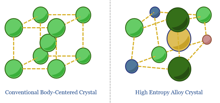
High entropy alloys: new metal?

High Entropy Alloys are an emerging class of materials, composed of five or more elements, forming fascinating/novel lattice structures. This 18-page report reviews 100 recent HEA patents, and predicts generative AI will unlock transformational catalysts and materials in the next decade.
-
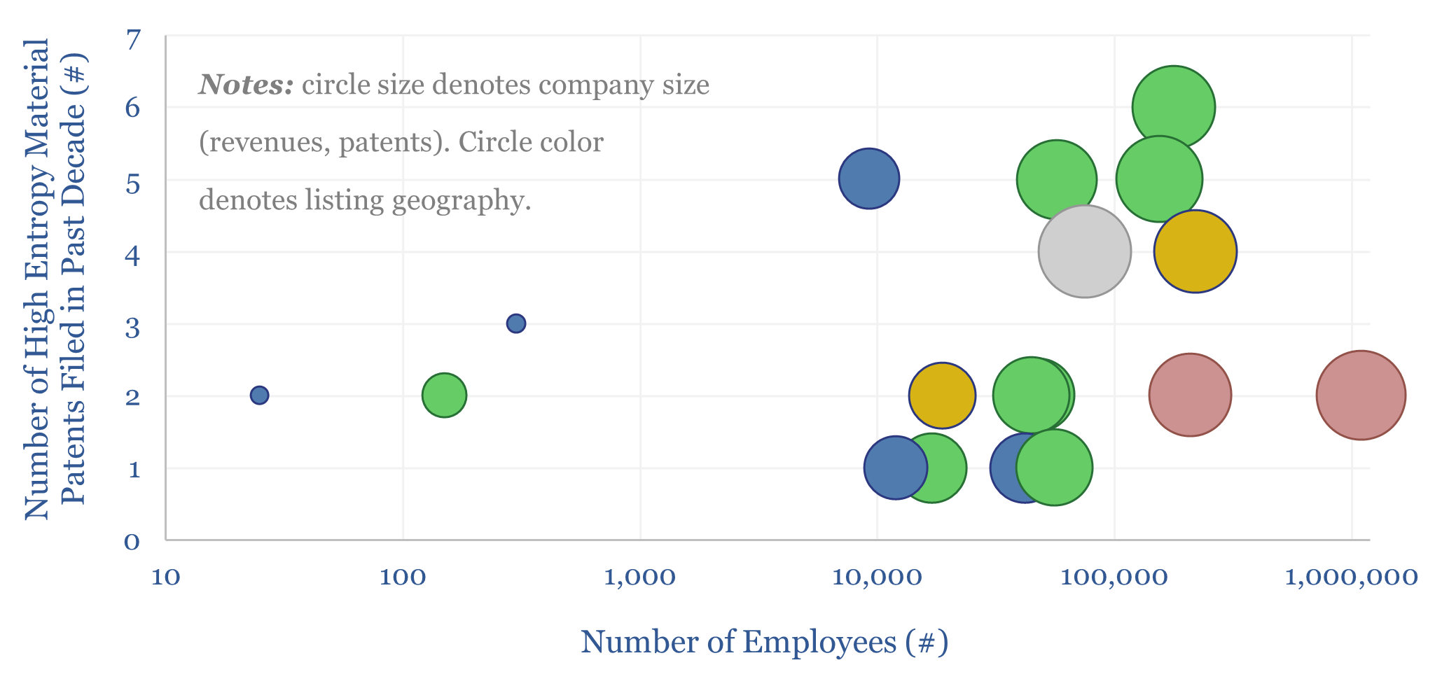
Leading companies in high entropy alloys?

This data-file evaluates 100 patents, filed over the past decade, by leading companies in high entropy alloys, and by academic institutions. 20 companies stood out, developing harder and more resistant tools for machining/drilling, alloys that can withstand extreme temperatures, and novel surface coatings.
-
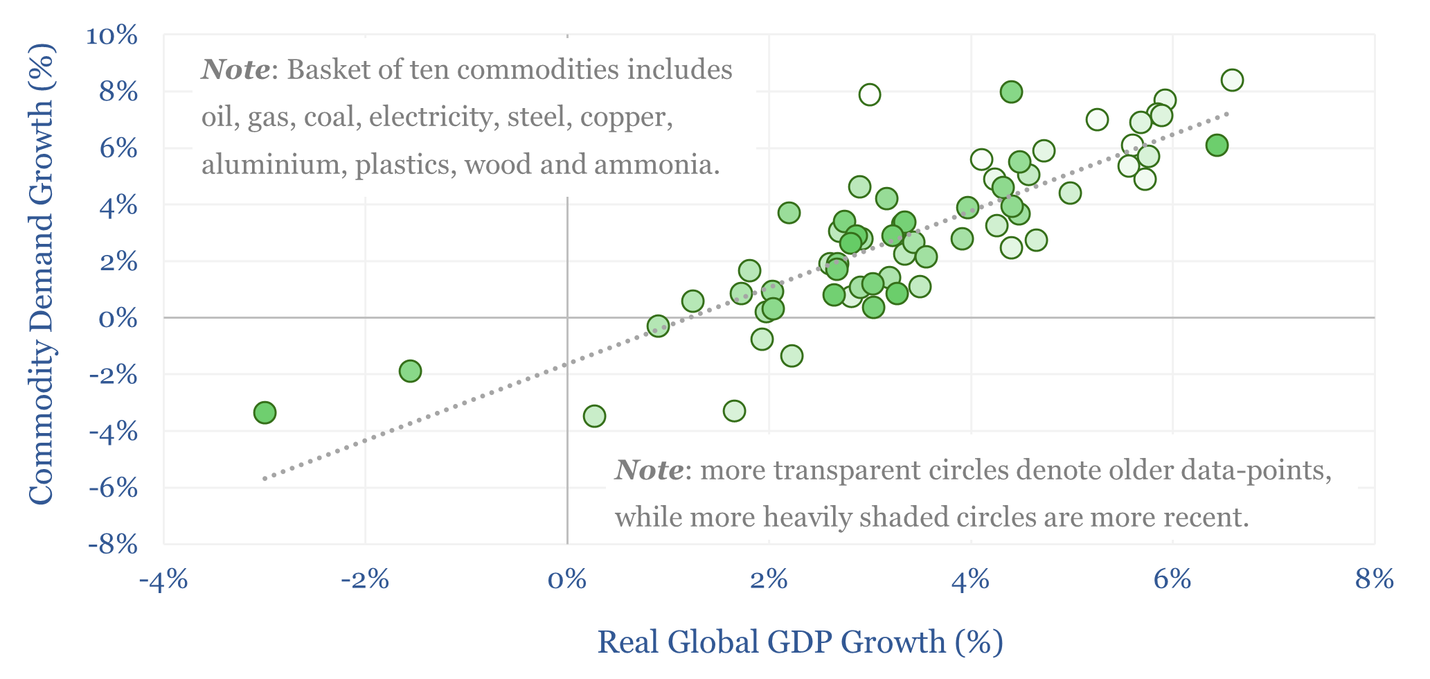
Global commodity demand: sensitivity to GDP?

Global commodity demand is levered to GDP. Specifically, for each +/- 1% acceleration or deceleration in global GDP, commodity demand tends to accelerate or decelerate by +/- 1.4%, with a 70% R-squared, across 25 examples that are indexed in this data-file. Oil demand sensitivity to GDP is particularly interesting.
-
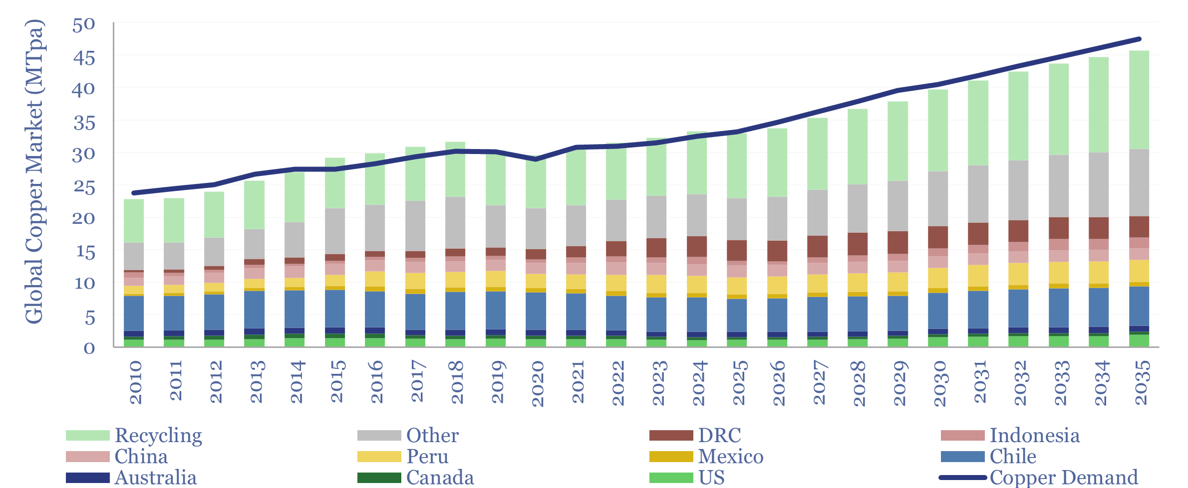
Global copper supply-demand

Global copper supply-demand is tabulated in this data-file, looking across 90 mines and upcoming projects, by country, and over time. Markets were 5% undersupplied when prices spiked in 2010-11, 6% over-supplied when they collapsed in 2015-16, and returned to undersupply in 2025. Undersupply persists through 2035, most likely at -3% pa, as demand grows by…
-
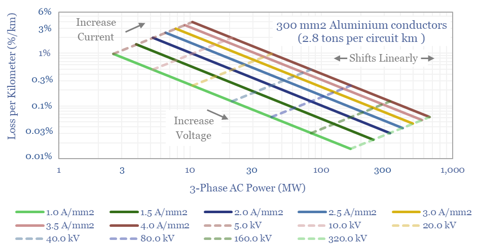
Power cables: carrying capacity and loss rates?

This data-file calculates the power carrying capacity of power cables, plus the resistive losses of power cables. Both are modeled as a function of their voltage, current density, copper and/or aluminium content, resistance and connection type. Underlying data are drawn from data we have tabulated on over 100 conductors, their ratings and costs.
-
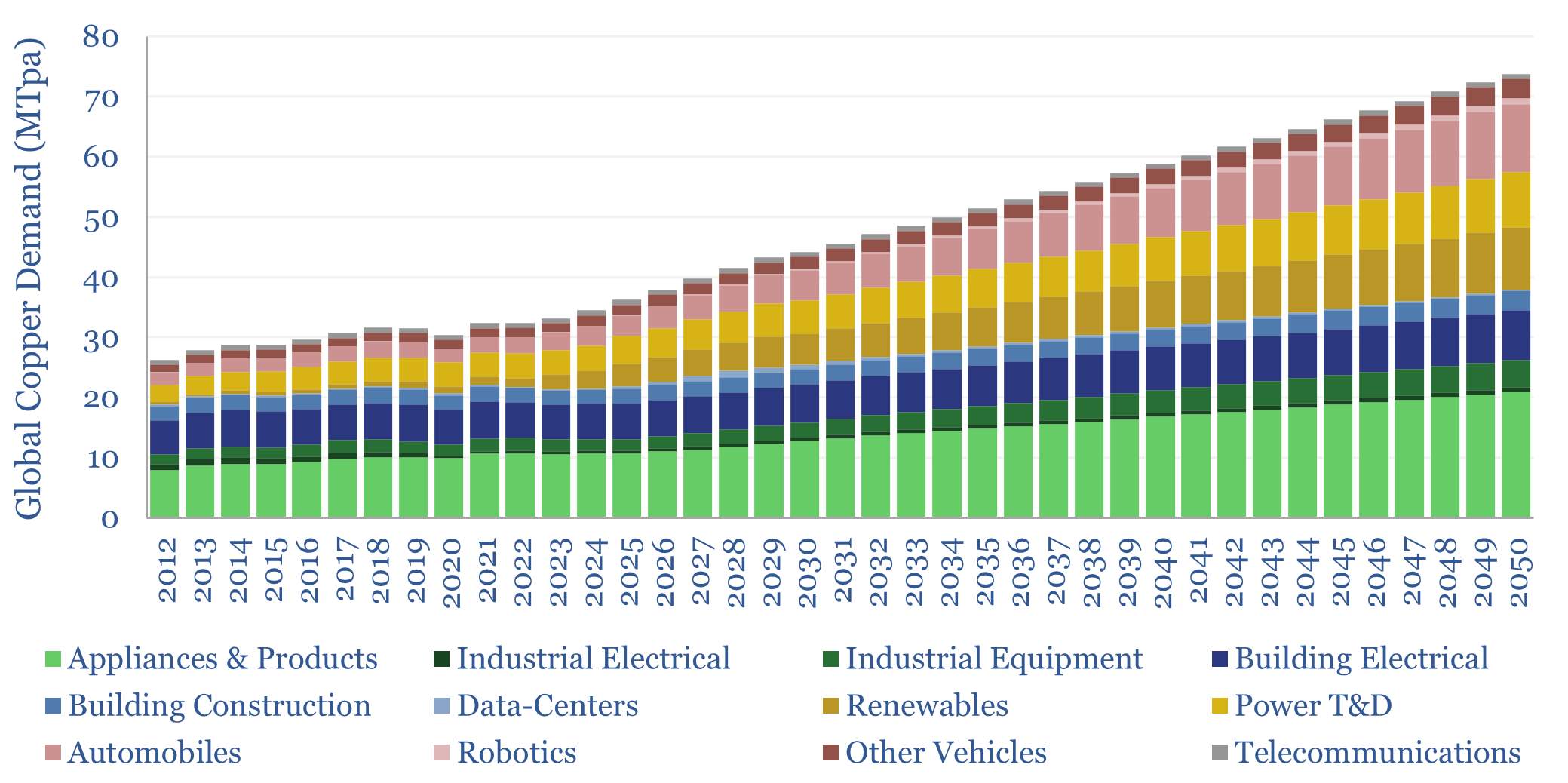
Copper: global demand forecasts?

This data-file estimates global copper demand as part of the energy transition, rising from 33MTpa in 2023 to 44MTpa in 2030 and 80MTpa by 2050. Key demand drivers are solar, EVs, greater AC adoption and possibly drones and robotics. You can stress test half-a-dozen key input variables in the model.
-
Global lithium production: by project, by country, by resource?

Global lithium production, by project, by country, by resource type, and over time, are aggregated in this data-file, by tabulating details of each project. There is spare capacity in 2026, especially from Australian mine projects, but the current project pipeline sugggests a 20-30% market deficit in 2030-35.

Content by Category
- Batteries (96)
- Biofuels (44)
- Carbon Intensity (48)
- CCS (64)
- CO2 Removals (9)
- Coal (44)
- Commentary (65)
- Company Diligence (105)
- Data Models (927)
- Decarbonization (162)
- Demand (131)
- Digital (89)
- Downstream (47)
- Economic Model (222)
- Energy Efficiency (76)
- Hydrogen (63)
- Industry Data (310)
- LNG (56)
- Materials (86)
- Metals (89)
- Midstream (45)
- Natural Gas (163)
- Nature (76)
- Nuclear (28)
- Oil (178)
- Patents (39)
- Plastics (44)
- Power Grids (156)
- Renewables (153)
- Screen (138)
- Semiconductors (35)
- Shale (58)
- Solar (72)
- Supply-Demand (53)
- Vehicles (94)
- Video (24)
- Wind (46)
- Written Research (409)