Coal
-
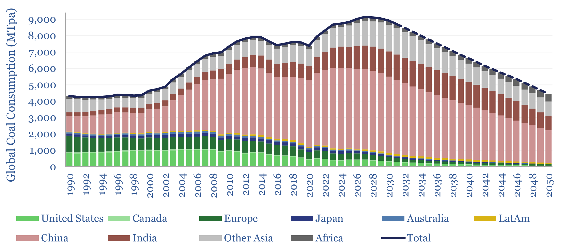
Global coal supply-demand: outlook in energy transition?

Global coal supply-demand remained at all-time peak levels of 8.8GTpa in 2025, of which 7.6GTpa is thermal coal and 1.1GTpa is metallurgical. The largest consumers are China (4.9GTpa), India (1.3GTpa), other Asia (1.3GTpa), Europe (0.4GTpa) and the US (0.4GTpa). This model presents our forecasts for global coal supply-demand from 1990 to 2050.
-
Global hydrocarbon resources: across the history of the world?
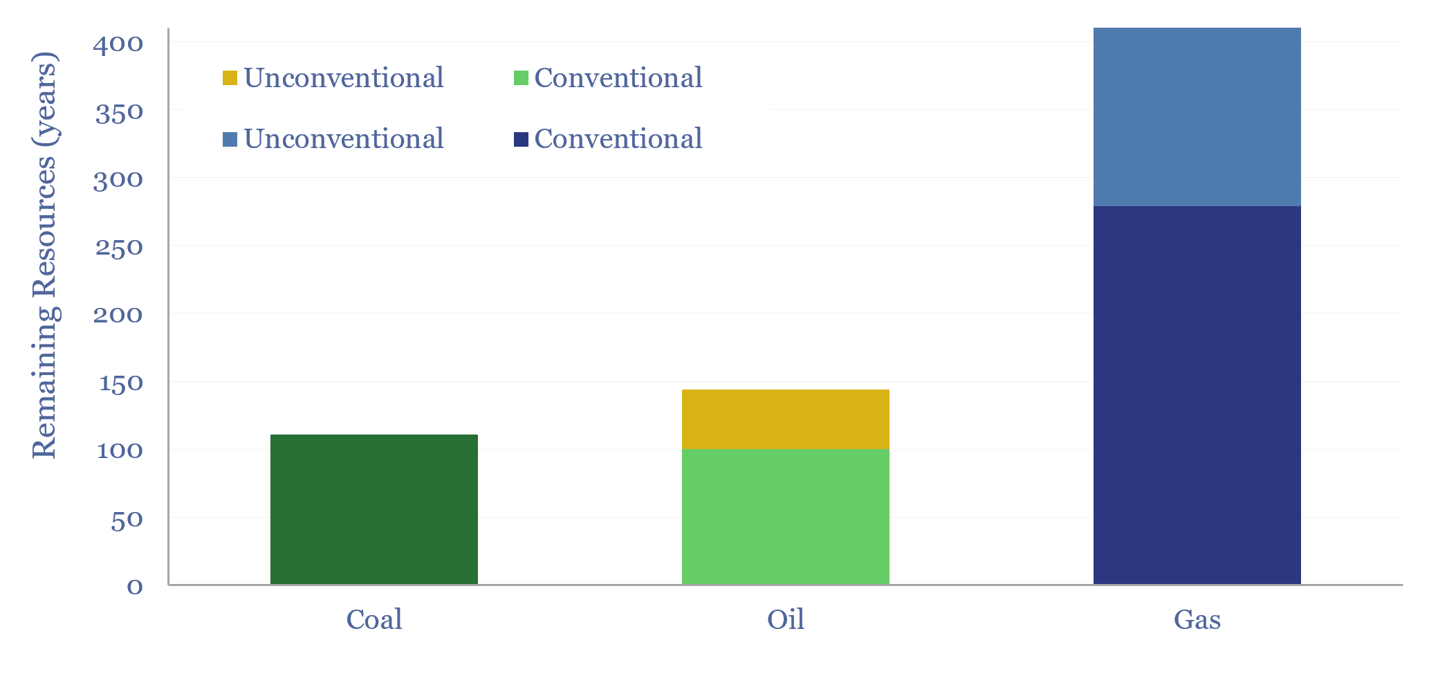
We have quantified global hydrocarbon resources, from first principles, in this 15-page report. We estimate how much oil, gas and coal ever formed across the total history of the world. And more importantly, we estimate how much is left. Our numbers support an energy transition from coal to gas.
-
Global hydrocarbon resources and coal resources?
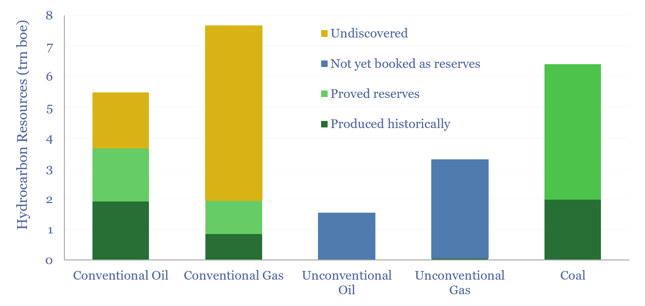
Global hydrocarbon resources and global coal resources — in-place resources and economically recoverable resources — are estimated from first principles in this data-file. We see the world’s remaining economically recoverable reserves of oil and gas being 4x larger than remaining economically recoverable reserves of coal.
-
Tunnel boring: the economics?

The global market for tunnel boring machines has been estimated at $7.5bn pa. But what are the costs of tunnel boring? This data-file models tunnel boring economics, estimated at $10M/km for civil infrastructure projects today, $30M/km for deep mine shafts, but will cheap solar and autonomous robots deflate costs?
-
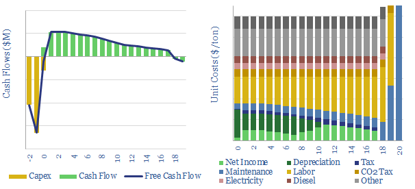
Coal mining: the economics?

The economics of coal mining are captured in this data-file. $60/ton coal, equivalent to 1c/kWh-th, at the bottom of the global energy cost curve, can typically be unlocked by capex costs of $60/Tpa at a new coal mine, and other opex costs, tabulated in the data-file.
-
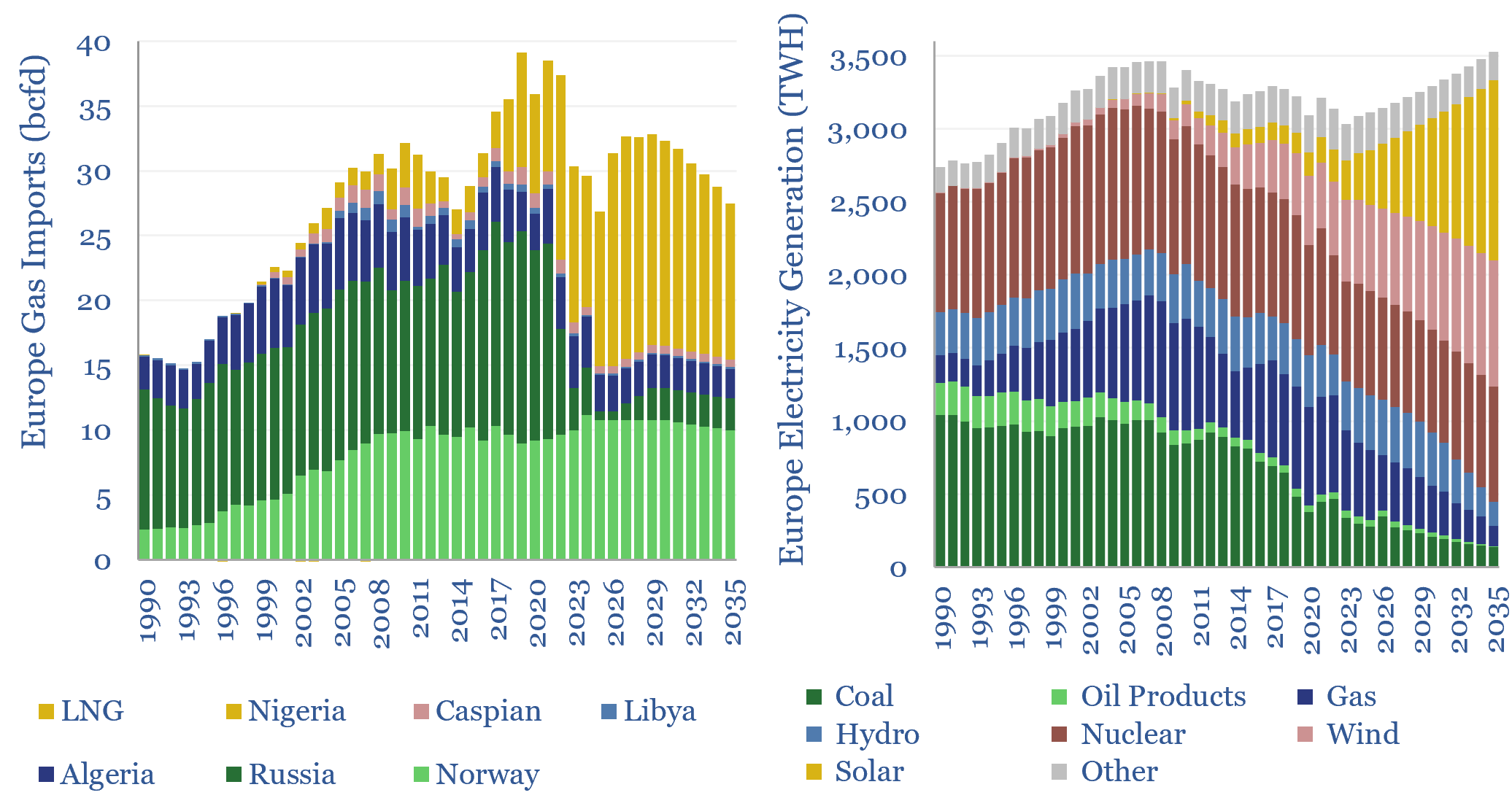
European gas and power model: natural gas supply-demand?

This data-file is our European gas supply-demand model. Balances are assessed in European gas and power markets from 1990 to 2035, reflecting all of our research into Europe’s energy transition. 2024-25 gas markets were supported by inventory draw-downs, but LNG imports step up from 110MTpa to 120MTpa through 2030, before softening again through 2035.
-
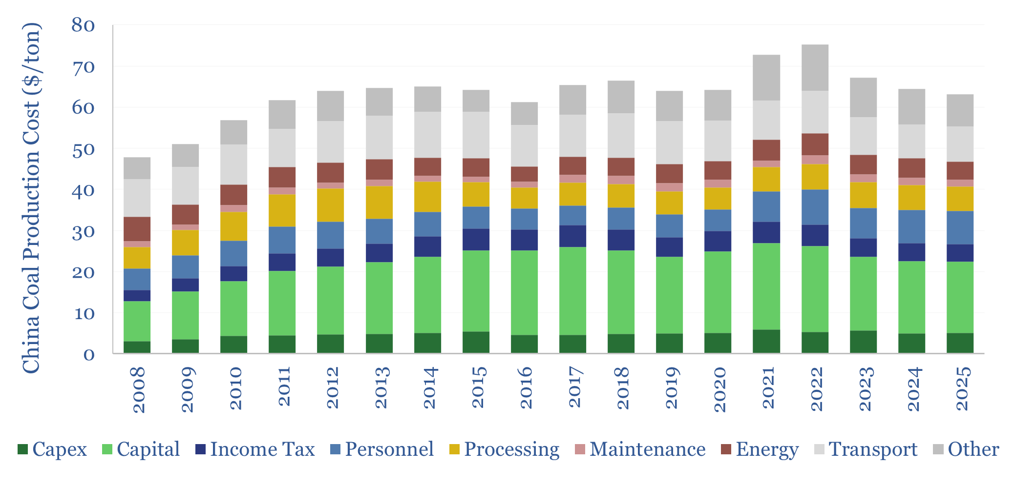
China coal production costs?

China coal production costs are estimated on a full-cycle basis in this data-file, averaging $65/ton across large, listed miners, with assets in Shanxi, Inner Mongolia and Shaanxi, and 1.5-2x higher again for smaller regional prices. The costs had been increasing at $1.3/ton/year through 2023, but moderated in 2024-25. But could marginal Chinese coal prices hit…
-
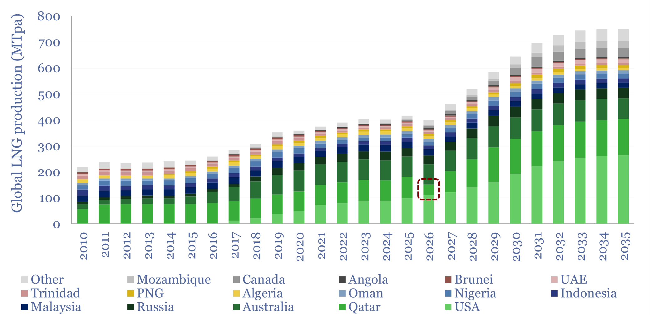
Qatari LNG: the worst supply disruption in LNG history?

What if Qatar’s LNG output falls by -50% YoY in 2026, i.e., by -40MTpa, which is equivalent to a -0.4% reduction in useful global energy supplies? This 11-page report revisits all of our regional energy models, predicts how each Qatari LNG customer will fill the shortfall, and the implications for global energy markets.
-
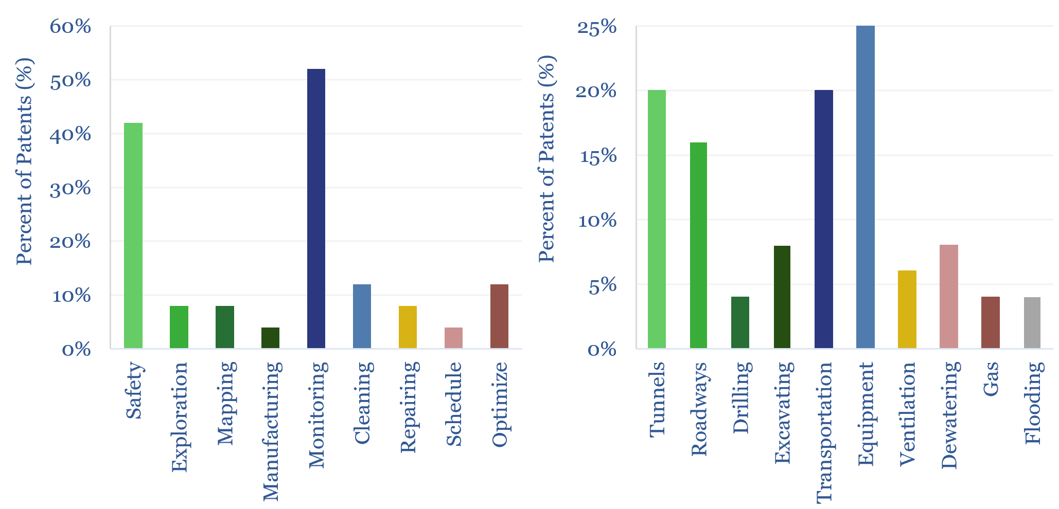
Are AI and robotics deflating coal costs?

This data-file tracks the progress in deploying AI in the coal industry, and deploying robots in the coal industry, based on the evidence from patents filed in 2025 and early 2026. AI is increasingly under study, but mainly for safety and monitoring applications, and often specifically to combat resource depletion, which is discussed in c30%…
-
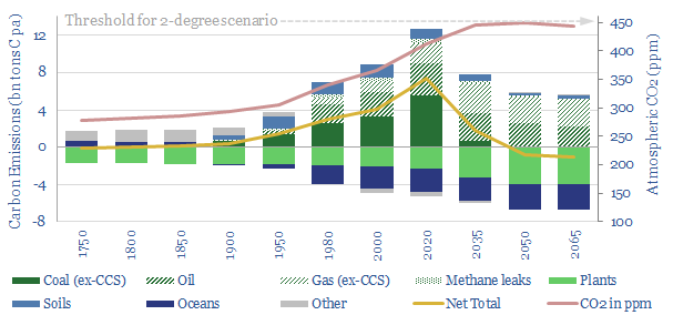
The route to net zero: an energy-climate model for 2-degrees

We have modeled the global climate system from 1750-2065, to simplify the science of energy transition. ‘Net zero’ is achievable by 2050. Atmospheric CO2 remains below 450ppm, consistent with 2-degrees warming. Fossil fuel usage is 10% higher than today, but the fossil fuel industry is transformed.
Content by Category
- Batteries (96)
- Biofuels (44)
- Carbon Intensity (48)
- CCS (64)
- CO2 Removals (9)
- Coal (44)
- Commentary (65)
- Company Diligence (105)
- Data Models (928)
- Decarbonization (163)
- Demand (131)
- Digital (92)
- Downstream (47)
- Economic Model (222)
- Energy Efficiency (76)
- Hydrogen (63)
- Industry Data (311)
- LNG (56)
- Materials (86)
- Metals (89)
- Midstream (45)
- Natural Gas (163)
- Nature (76)
- Nuclear (28)
- Oil (178)
- Patents (39)
- Plastics (44)
- Power Grids (156)
- Renewables (153)
- Screen (139)
- Semiconductors (36)
- Shale (58)
- Solar (72)
- Supply-Demand (53)
- Vehicles (94)
- Video (24)
- Wind (46)
- Written Research (410)