Vehicles
-
Vehicles: energy transition conclusions?
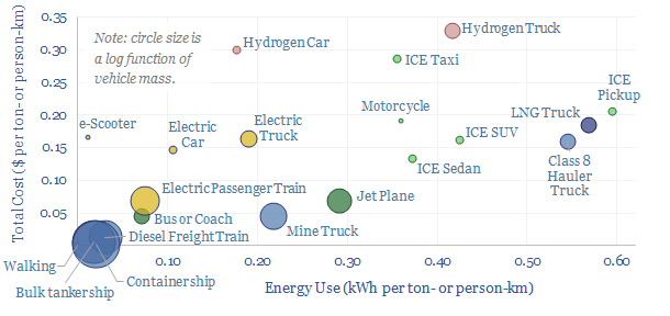
Vehicles transport people and freight around the world, explaining 70% of global oil demand, 30% of global energy use, 20% of global CO2e emissions. This overview summarizes all of our research into vehicles, and key conclusions for the energy transition.
-
Passenger cars: what electrical loads in vehicles?
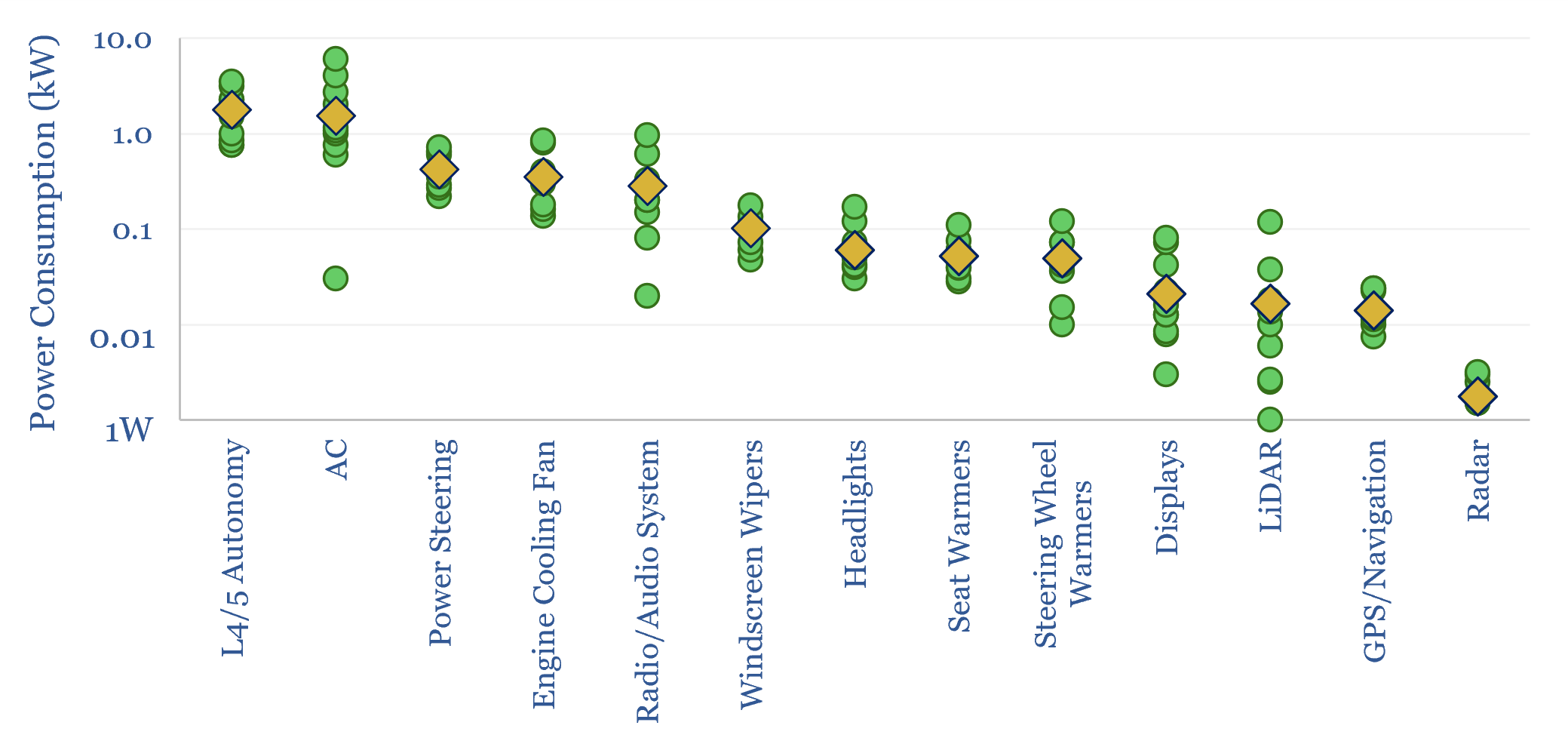
Electrical loads in vehicles typically average 1kW, in order to power HVAC, computers, engine cooling, steering, sensors and entertainment. This equates to 500TWH of electricity demand globally within ICEs, even before considering electrification. Fully autonomous vehicles would likely consume another 1-3kW again for on-board AI chips.
-
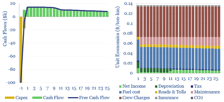
Heavy truck costs: diesel, gas, electric or hydrogen?

Heavy truck costs are estimated at $0.14 per ton-kilometer, for a truck typically carrying 15 tons of load and traversing over 150,000 miles per annum. Today these trucks consume 10Mbpd of diesel and their costs absorb 4% of post-tax incomes. Hydrogen trucks would be 45-75% more costly, but from 2026, we are starting to see…
-
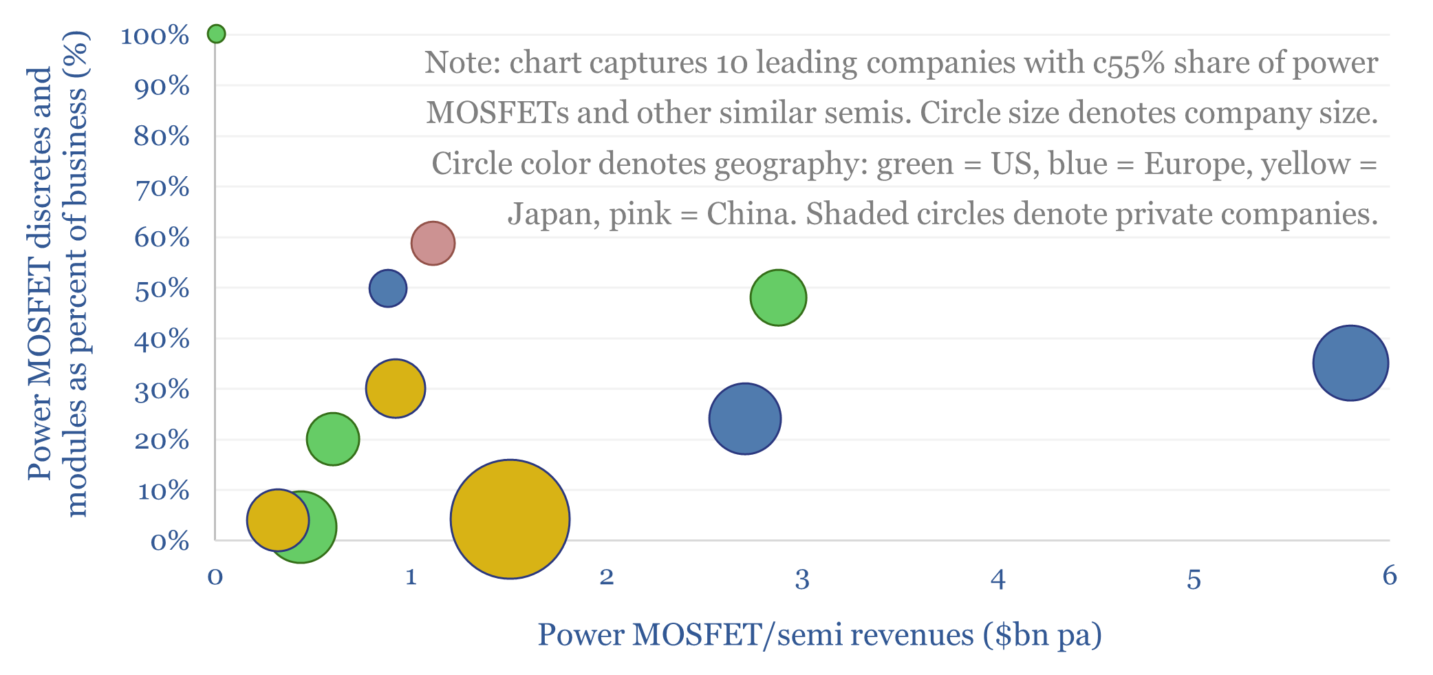
Power-MOSFETs: active semiconductor companies?

Power MOSFETs are an energy transition technology, the building block behind inverters, DC-DC converters, EV drive trains, EV chargers, renewables-battery interfaces and increasingly, the power conversion architectures for upscaling rack density at AI data-centers. Hence this data-file is a screen of power MOSFET and active semiconductor companies.
-
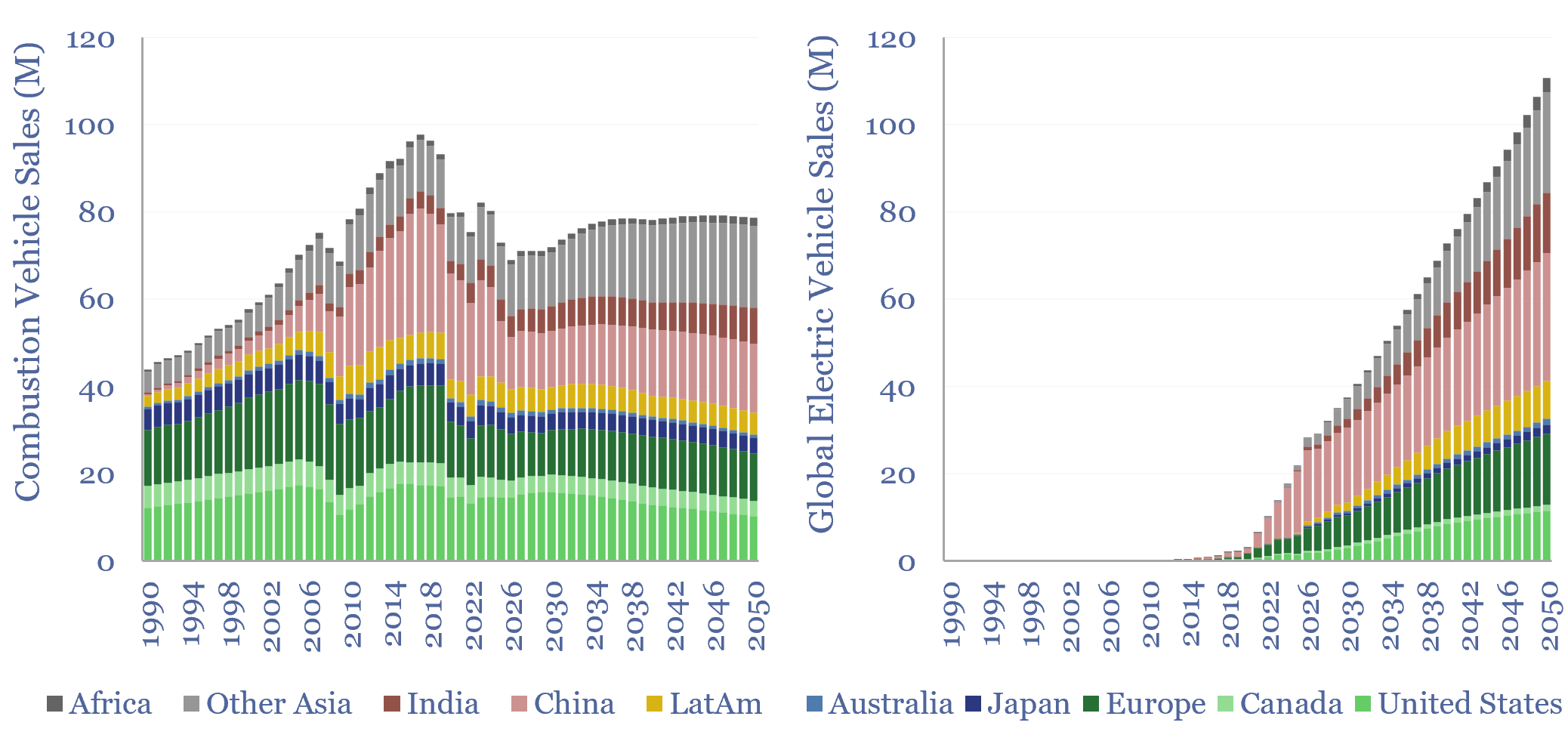
Global vehicle fleet: vehicle sales and electrification by region?

Global electric vehicle sales will ramp from c22M units in 2025 to 120M units in 2050, while combustion vehicle sales run flat at 80M units per year. This data-file forecasts global electric vehicle sales by region, the total electric vehicle fleet, and thus informs our models for long-term global oil demand.
-
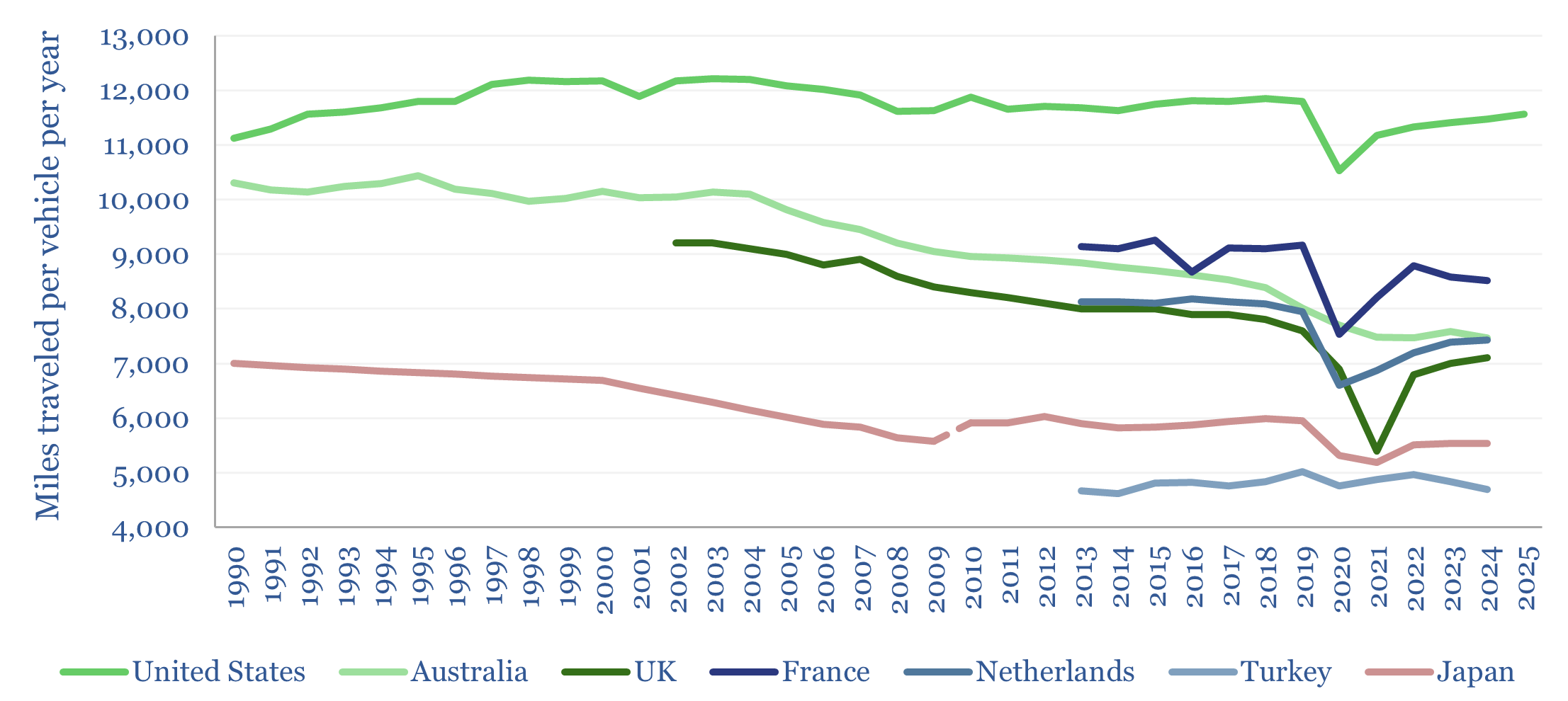
Vechile miles traveled by region over time?

Vehicle miles traveled are a crucial measure of mobility and an input variable for predicting global oil demand, averaging 8,600 miles per global vehicle in 2024. This data-file tracks vehicle miles traveled by region, over time, and how it co-varies with urbanization, population density, income, and by travel trip purpose.
-
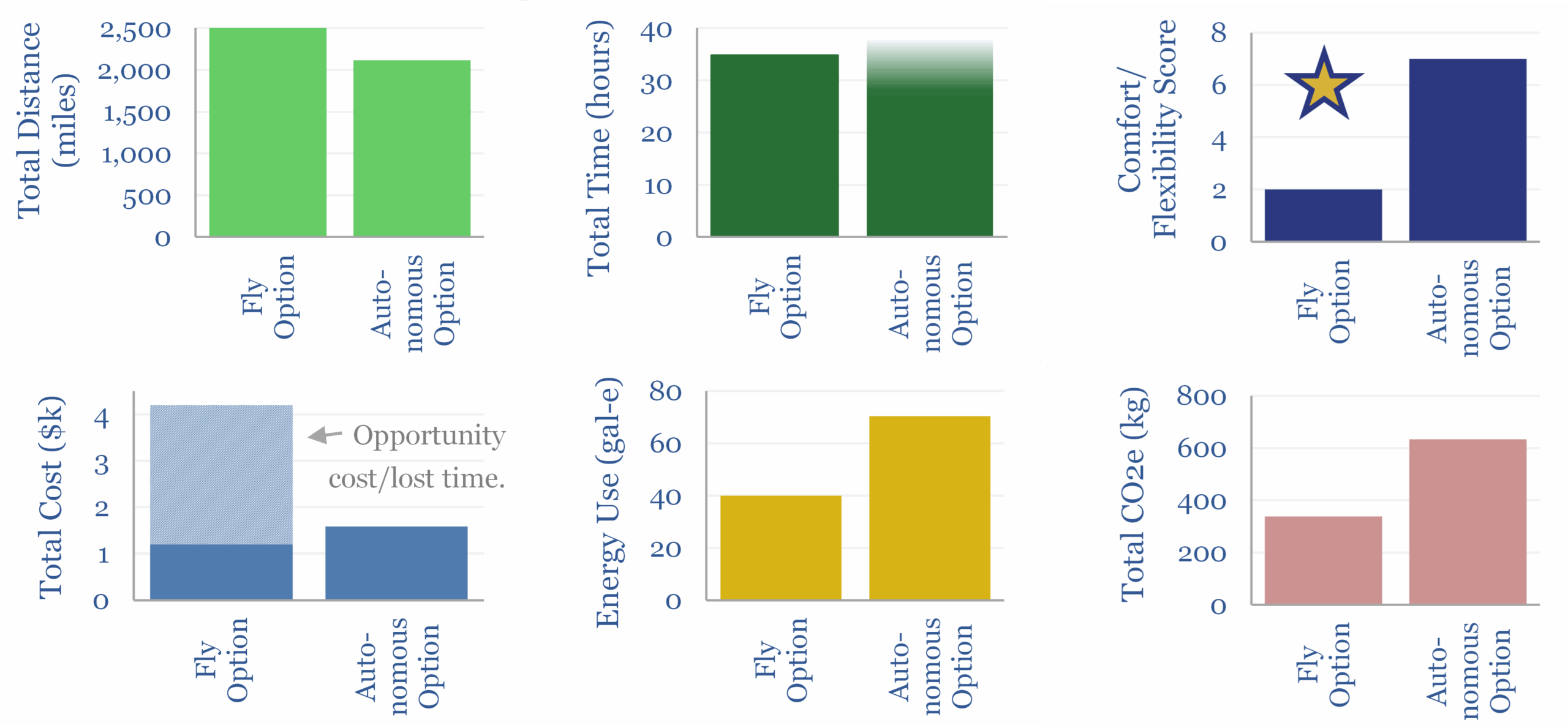
Autonomous transport: the Leipzig test?

This 13-page report explores the upside in autonomous transport. We were recently invited to a fascinating company event in Leipzig, Germany. But it was too complex to reach by flying. It would have been doable in an autonomous vehicle, albeit using 2x more energy overall. So could autonomous vehicles unlock 5Mbpd of global oil demand…
-
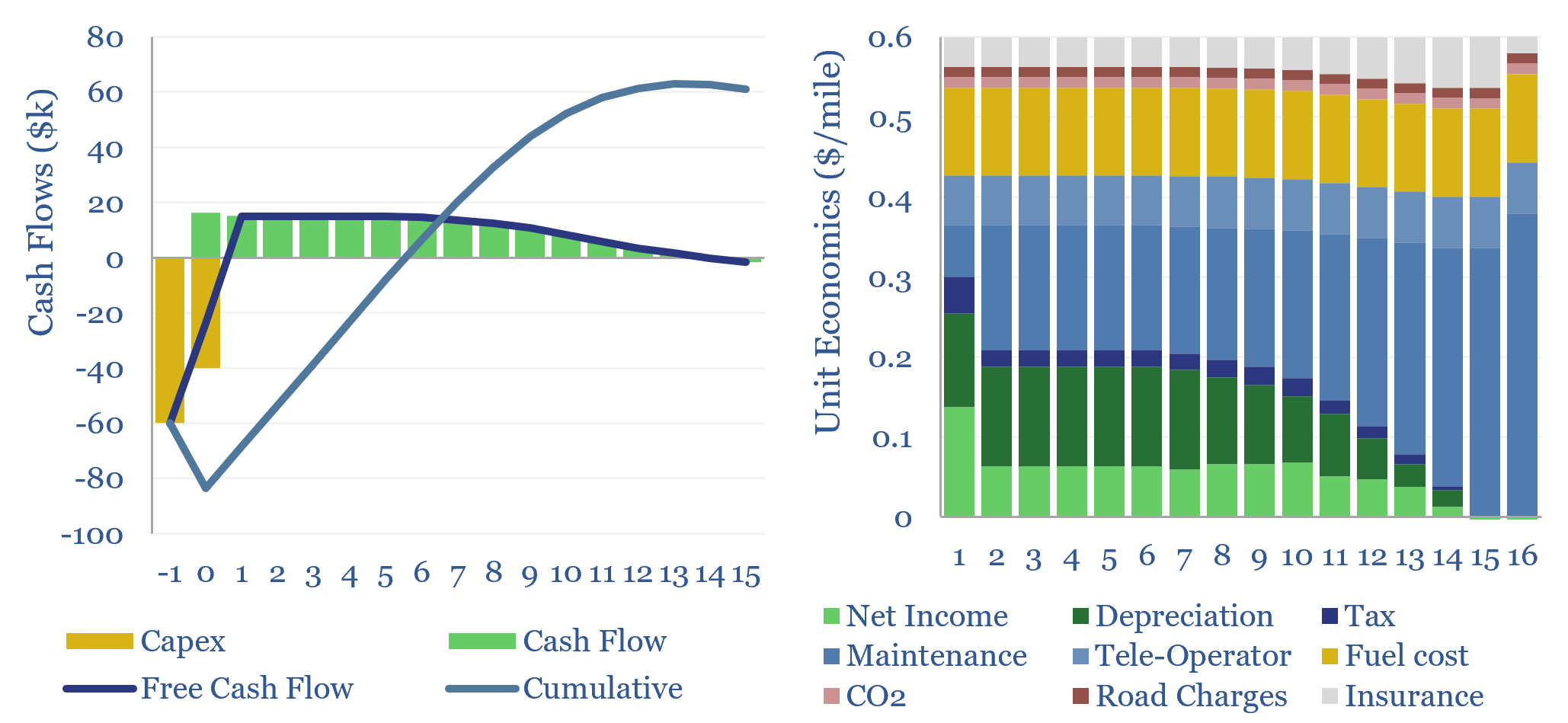
Autonomous vehicles: the economics?

This data-file explores the costs of autonomous vehicles. An autonomous vehicle traveling c100,000 miles per year, at 20% capacity utilization, must charge a fee of $0.6/mile, in order to generate a 10% IRR on c$100k of vehicle acquisition capex.
-
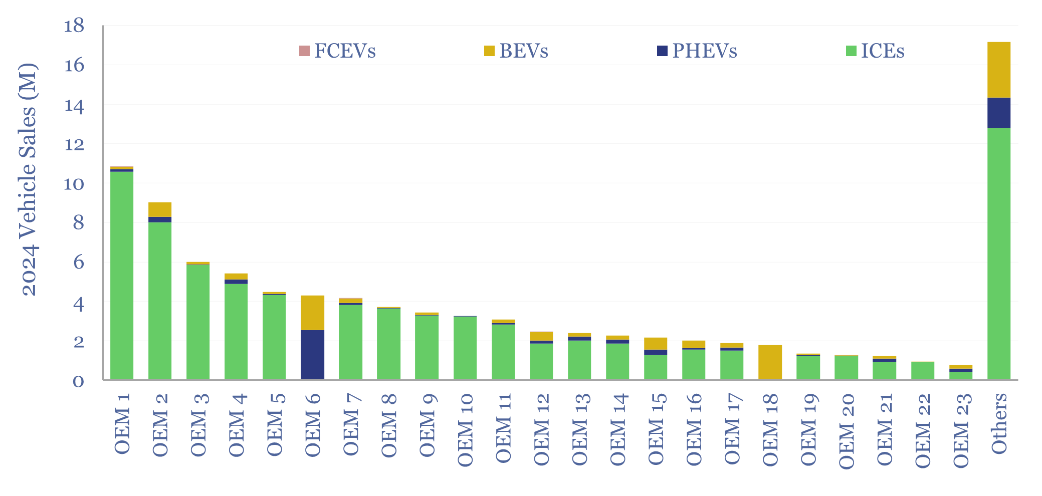
Global vehicle sales by manufacturer?

Global vehicle sales by manufacturer are broken down in this screen. 25 companies produce 85% of the world’s vehicles, led by Toyota, VW, Stellantis, GM and Ford. The data-file contains key notes on each company. In 2025, 35% of companies slowed their deployment of electric vehicles, while 95% accelerated their focus on autonomous vehicles.
-
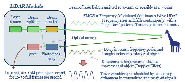
Autonomous-ready sensors: the LiDAR debate?

The sensors used for advanced driver assistance systems (ADAS), and increasingly for autonomous vehicles, offer useful lessons for AI, robotics and mining. Hence this 17-page report revisits the debate between LiDAR vs cameras, radar and ultrasound. Hardware must compete on cost and performance. But who benefits from deflation?
Content by Category
- Batteries (96)
- Biofuels (44)
- Carbon Intensity (48)
- CCS (64)
- CO2 Removals (9)
- Coal (44)
- Commentary (65)
- Company Diligence (105)
- Data Models (927)
- Decarbonization (163)
- Demand (131)
- Digital (90)
- Downstream (47)
- Economic Model (222)
- Energy Efficiency (76)
- Hydrogen (63)
- Industry Data (311)
- LNG (56)
- Materials (86)
- Metals (89)
- Midstream (45)
- Natural Gas (163)
- Nature (76)
- Nuclear (28)
- Oil (178)
- Patents (39)
- Plastics (44)
- Power Grids (156)
- Renewables (153)
- Screen (138)
- Semiconductors (35)
- Shale (58)
- Solar (72)
- Supply-Demand (53)
- Vehicles (94)
- Video (24)
- Wind (46)
- Written Research (409)