Supply-Demand
-
Global energy: supply-demand model?
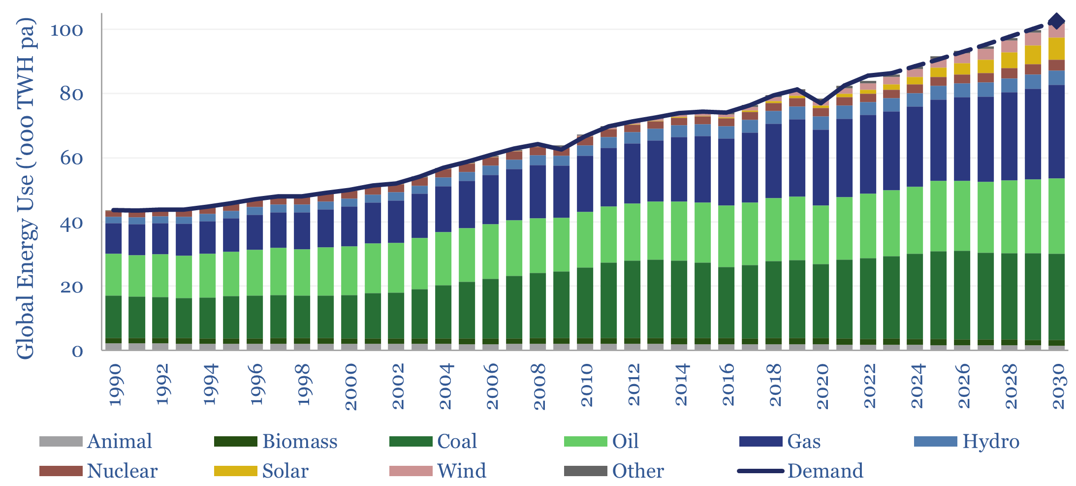
This global energy supply-demand model combines our supply outlooks for coal, oil, gas, LNG, wind and solar, nuclear and hydro, into a build-up of useful global energy balances in 2023-30. 2026 will be a year of recalibration, as global energy markets shift from c1% over-supply in 2025 to -0.5% under-supply in 2027?
-
Global plastic demand: breakdown by product, region and use?

Global plastic is estimated at 530MTpa in 2025, rising to 1GTpa by 2050. This data-file is a breakdown of global plastic demand, by product, by region and by end use, with historical data back to 1990 and our forecasts out to 2050. Our top conclusions for plastic demand, by region, by product, by fate, are…
-
Global gas supply-demand in energy transition?

Global gas supply-demand is predicted to rise from 400bcfd in 2023 to 650bcfd by 2050, in our outlook, as a complement to wind, solar, nuclear, and as global coal resources mature from the 2030s onwards. This data-file quantifies global gas demand and supply by country, across heating, power and industry.
-
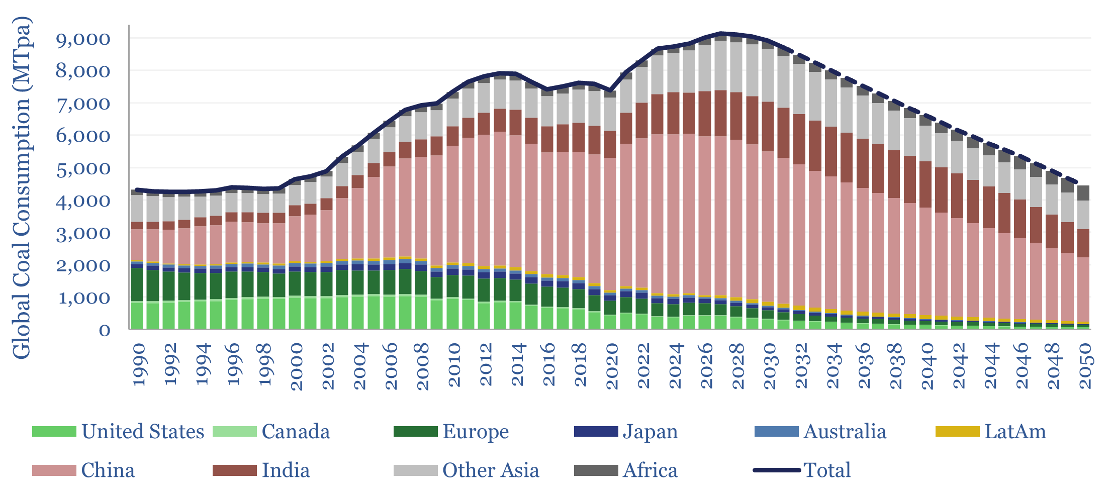
Global coal supply-demand: outlook in energy transition?

Global coal supply-demand remained at all-time peak levels of 8.8GTpa in 2025, of which 7.6GTpa is thermal coal and 1.1GTpa is metallurgical. The largest consumers are China (4.9GTpa), India (1.3GTpa), other Asia (1.3GTpa), Europe (0.4GTpa) and the US (0.4GTpa). This model presents our forecasts for global coal supply-demand from 1990 to 2050.
-
US shale: outlook and forecasts?

This model sets out our US shale production forecasts by basin. It covers the Permian, Bakken, Eagle Ford, Marcellus/Utica and Haynesville, as a function of the rig count, drilling productivity, completion rates, well productivity and type curves. The data-file was last updated in May-2025, revising liquids growth negative in 2025-26, which in turn tightens US…
-
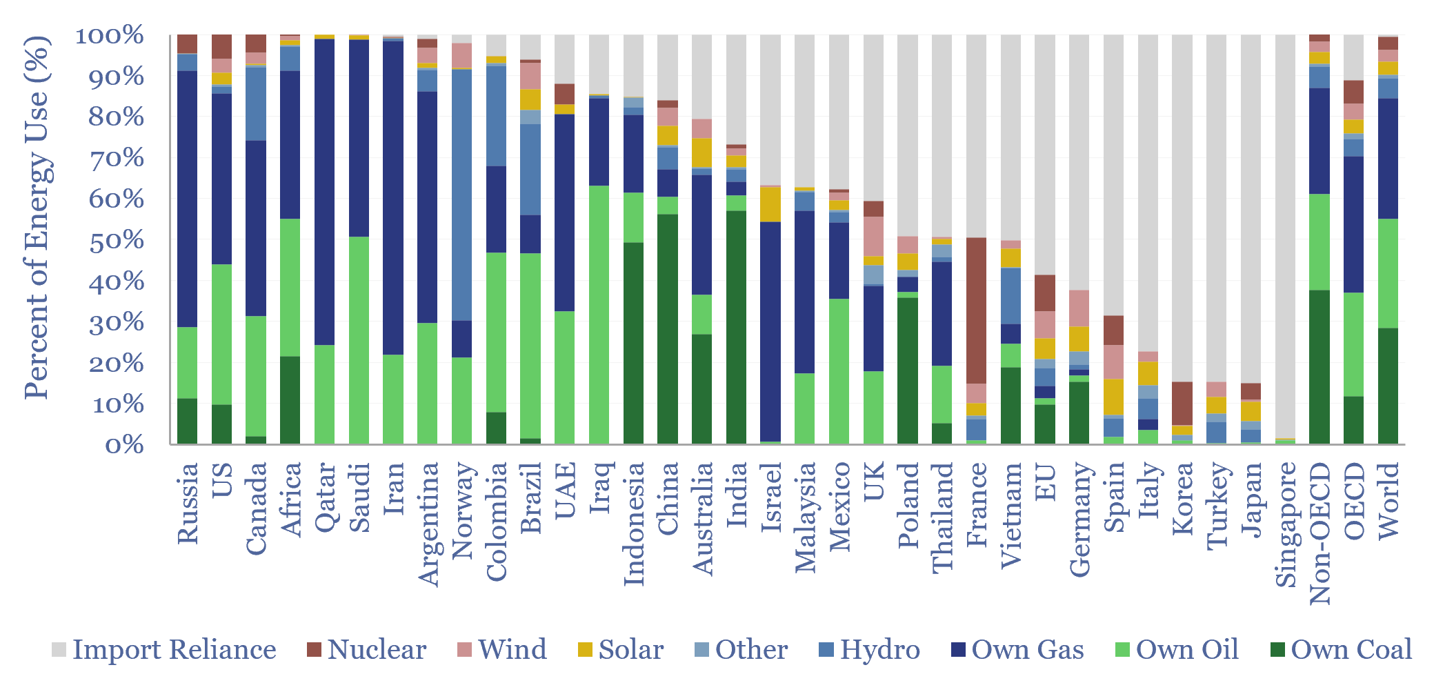
Energy self-sufficiency by country and over time?

This data-file tabulates energy self-sufficiency, by country, over time, across 30 of the largest economies in the world. Among this sample, the median country generates 70% of its energy domestically, and is reliant on imports for 30% of the remainder. Energy self-sufficiency varies vastly by country.
-
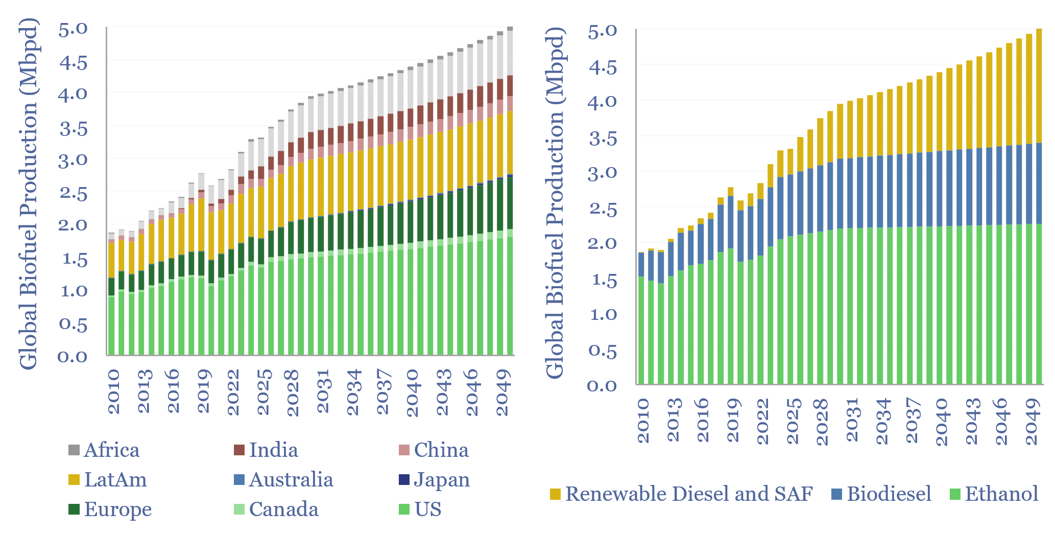
Global biofuel production: by region, by liquid fuel?

Global liquid biofuel production ran at 3.3Mbpd in 2025, of which c60% is ethanol, c30% is biodiesel and c10% is renewable diesel. 65% of global production is from the US and Brazil. Our forecasts for global liquid biofuel production reach 3.8Mbpd by 2030 and 5Mbpd by 2050, with 75% of the growth in renewable diesel.
-
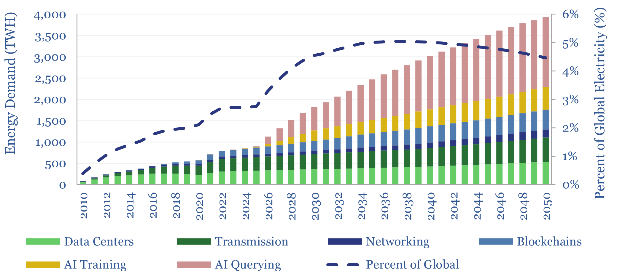
Internet energy consumption: data, models, forecasts?

This data-file forecasts the energy consumption of the internet, rising from 800 TWH in 2022 to 2,000 TWH in 2030 and over 4,000 TWH by 2050. The main driver is the energy consumption of AI, plus blockchains, rising traffic, and offset by rising efficiency. Input assumptions to the model can be flexed. Underlying data are…
-
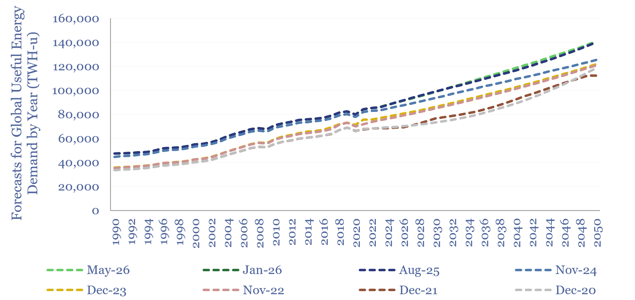
Energy supply-demand forecast revisions over time?

This data-file captures the forecast revisions, over time, in our various energy supply-demand models. Over the past seven years, we have consistently and enormously increased our forecasts for solar and coal. We have also repeatedly raised our forecasts for global oil and electricity use. Conversely, we have seen slower growth in gas and EVs, and…
-
Global electricity: by source, by use, by region?

Global electricity supply-demand is disaggregated in this data-file, by source, by use, by region, from 1990 to 2050, triangulating across all of our other models in the energy transition, and culminating in over 50 fascinating charts, which can be viewed in this data-file. Global electricity demand rises 3x by 2050 in our outlook.


Content by Category
- Batteries (96)
- Biofuels (44)
- Carbon Intensity (48)
- CCS (64)
- CO2 Removals (9)
- Coal (44)
- Commentary (65)
- Company Diligence (105)
- Data Models (929)
- Decarbonization (163)
- Demand (132)
- Digital (92)
- Downstream (47)
- Economic Model (222)
- Energy Efficiency (76)
- Hydrogen (63)
- Industry Data (311)
- LNG (56)
- Materials (86)
- Metals (89)
- Midstream (45)
- Natural Gas (163)
- Nature (76)
- Nuclear (28)
- Oil (178)
- Patents (39)
- Plastics (44)
- Power Grids (157)
- Renewables (153)
- Screen (139)
- Semiconductors (36)
- Shale (58)
- Solar (73)
- Supply-Demand (53)
- Vehicles (94)
- Video (24)
- Wind (46)
- Written Research (410)