Midstream
-
Midstream opportunities in the energy transition?
The midstream industry moves molecules, especially energy-molecules, and especially in pipelines. Despite the mega-trend of electrification, there are still strong midstream opportunities in the energy transition, backstopping volatility and moving new molecules. This short note captures our top ten conclusions.
-
US shale: outlook and forecasts?

This model sets out our US shale production forecasts by basin. It covers the Permian, Bakken, Eagle Ford, Marcellus/Utica and Haynesville, as a function of the rig count, drilling productivity, completion rates, well productivity and type curves. The data-file was last updated in May-2025, revising liquids growth negative in 2025-26, which in turn tightens US…
-
Pipeline costs: moving oil, products or other liquids?
Pipeline costs are modeled in this data-file. $1/bbl is needed to move oil, oil products and other liquid commodities around 500 km at Mbpd scale, and the energy requirements are around 2.1 kWh/bbl, emitting 0.8 kg/bbl of CO2. Economics of scale matter. As a rule of thumb, costs rise by 100% when volumes fall by…
-
Compressor costs: a simple overview?
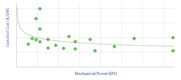
This data-file aims to give a helpful, basic overview of the $40bn pa compressor market, between centrifugal, reciprocating and screw compressors. A typical industrial unit is 50kW and costs $850/kW on an installed basis. Companies and efficiency calculations are also given.
-
Global gas prices: by country?

Global gas prices by country are often measured at the world-famous delivery points for liquids futures contracts, such as Henry Hub and the Netherlands’ TTF. This data-file takes a broader approach, aggregating the annual gas prices by country across twenty geographies.
-
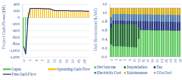
Gas storage: the economics?
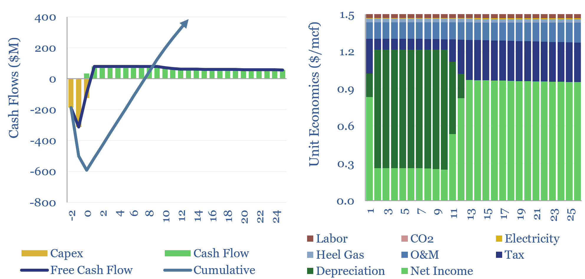
Gas storage economics are captured in this data-file. In our base case, a 30bcf underground storage facility, which cycles 2mcf per year of gas per mcf of gas capacity, requires a storage spread of $1.5/mcf to generate a 10% IRR off $19/mcf of capex. Effectively, this is inter-seasonal energy storage for 0.5c/kWh-th.
-
US LPG exports: the economics?

This data-file captures the economics of LPG exports, ethane exports, and/or propane exports from North America to Europe and Asia. Capex costs of LPG exports are c50% below LNG. Recent pricing underpins project-level c30% IRRs. The project pipeline is growing, but the data in this model of LPG exports do suggest strong returns for existing…
-
Container freight: shipping economics?
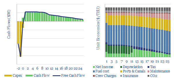
This data-file models the total costs of shipping a container c10,000 nautical miles from China to the West, in a 20,000 TEU vessel. Emerging fuels can lower the CO2 intensity of shipping from their baseline of 0.15kg/TEU-mile, by 60-90%, but freight costs inflate by 30%-3x.
-
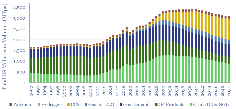
US gas pipeline capex over time?
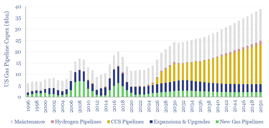
US gas pipeline capex ran at $12bn pa in 2023, but likely needs to treble to reach net zero by 2050, mainly to support 1GTpa of CCS. Midstream capex for natural gas, CO2 transportation and hydrogen production are forecast out to 2050 in this data-file. Numbers can be stress-tested in the model.
-
Midstream gas: pipelines have pricing power ?!
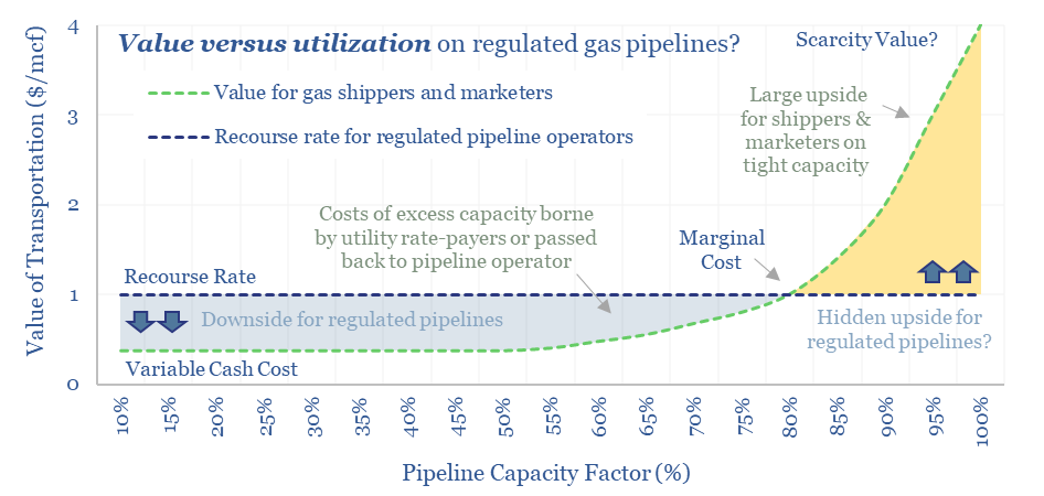
FERC regulations are surprisingly interesting!! In theory, gas pipelines are not allowed to have market power. But they increasingly do have it: gas use is rising, on grid bottlenecks, volatile renewables and AI; while new pipeline investments are being hindered. So who benefits here? Answers are explored in this 13-page report.
Content by Category
- Batteries (96)
- Biofuels (44)
- Carbon Intensity (48)
- CCS (64)
- CO2 Removals (9)
- Coal (44)
- Commentary (65)
- Company Diligence (106)
- Data Models (932)
- Decarbonization (163)
- Demand (132)
- Digital (92)
- Downstream (47)
- Economic Model (223)
- Energy Efficiency (76)
- Hydrogen (63)
- Industry Data (312)
- LNG (56)
- Materials (86)
- Metals (91)
- Midstream (45)
- Natural Gas (163)
- Nature (76)
- Nuclear (28)
- Oil (179)
- Patents (39)
- Plastics (44)
- Power Grids (157)
- Renewables (153)
- Screen (139)
- Semiconductors (36)
- Shale (58)
- Solar (73)
- Supply-Demand (53)
- Vehicles (94)
- Video (24)
- Wind (47)
- Written Research (411)