Economic Model
-
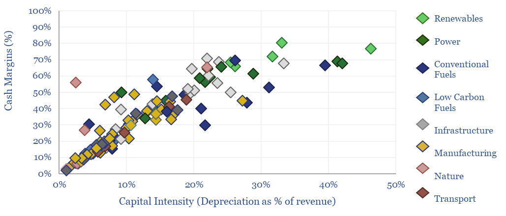
Energy economics: an overview?

This data-file provides an overview of energy economics, across 175 different economic models constructed by Thunder Said Energy, in order to put numbers in context. This helps to compare marginal costs, capex costs, energy intensity, interest rate sensitivity, and other key parameters that matter in the energy transition.
-
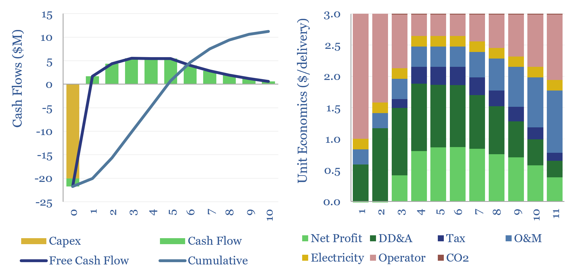
Costs of delivery drones: the energy economics?

The energy economics of delivery drones, which can travel autonomously, over 30km at 100kmph, are captured in this data-file. In our base case, a delivery drone that cost $20k, and makes 8 deliveries per day, must charge a fee of $3/delivery to generate a 10% IRR. Costs, speeds and energy use can be 5-20x superior…
-
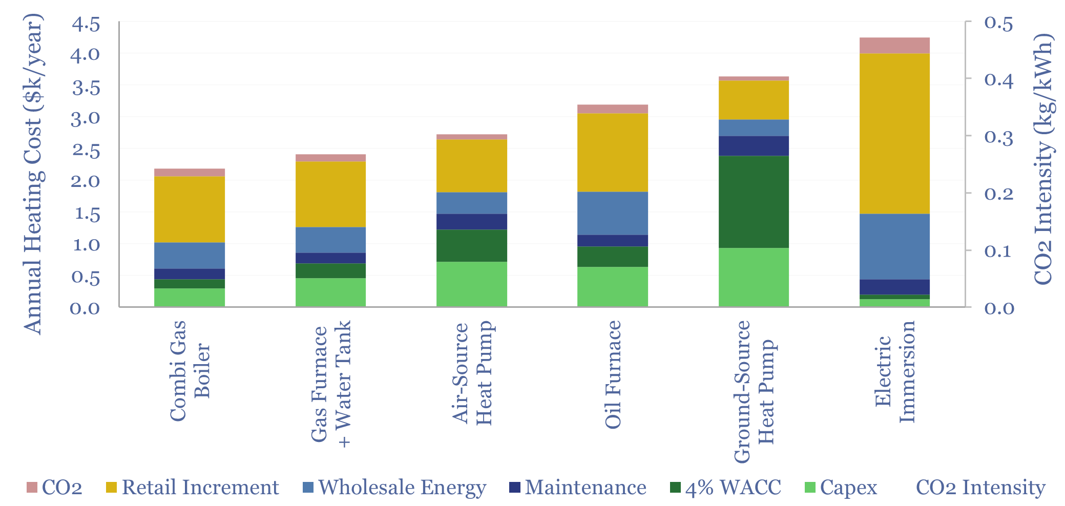
Residential heating costs: boilers, furnaces, electric and heat pumps?

Residential heating costs are compared and contrasted in this data-file, for gas-fired combi boilers, gas furnaces and hot water tanks, oil furnaces and hot water tanks, purely electric heating systems including immersion heaters, air-source heat pumps and ground-source heat pumps. Capex, maintenance and input energy prices can be stress-tested.
-
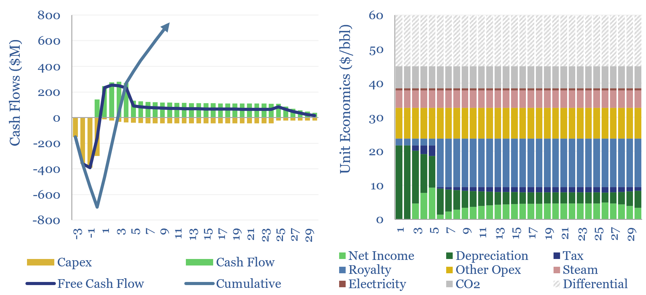
SAGD oil sands economics?

SAGD oil sands economics are modeled in this data-file, generating a 10% IRR, at $60/bbl WTI oil prices in our base case. This hinges on a 2.7 m3/m3 steam oil ratio, for a 4x EROEI. Breakevens can vary from $45-90/bbl depending on capex costs and steam oil ratios.
-
Coal mining: the economics?

The economics of coal mining are captured in this data-file. $60/ton coal, equivalent to 1c/kWh-th, at the bottom of the global energy cost curve, can typically be unlocked by capex costs of $60/Tpa at a new coal mine, and other opex costs, tabulated in the data-file.
-
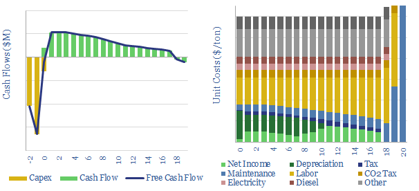
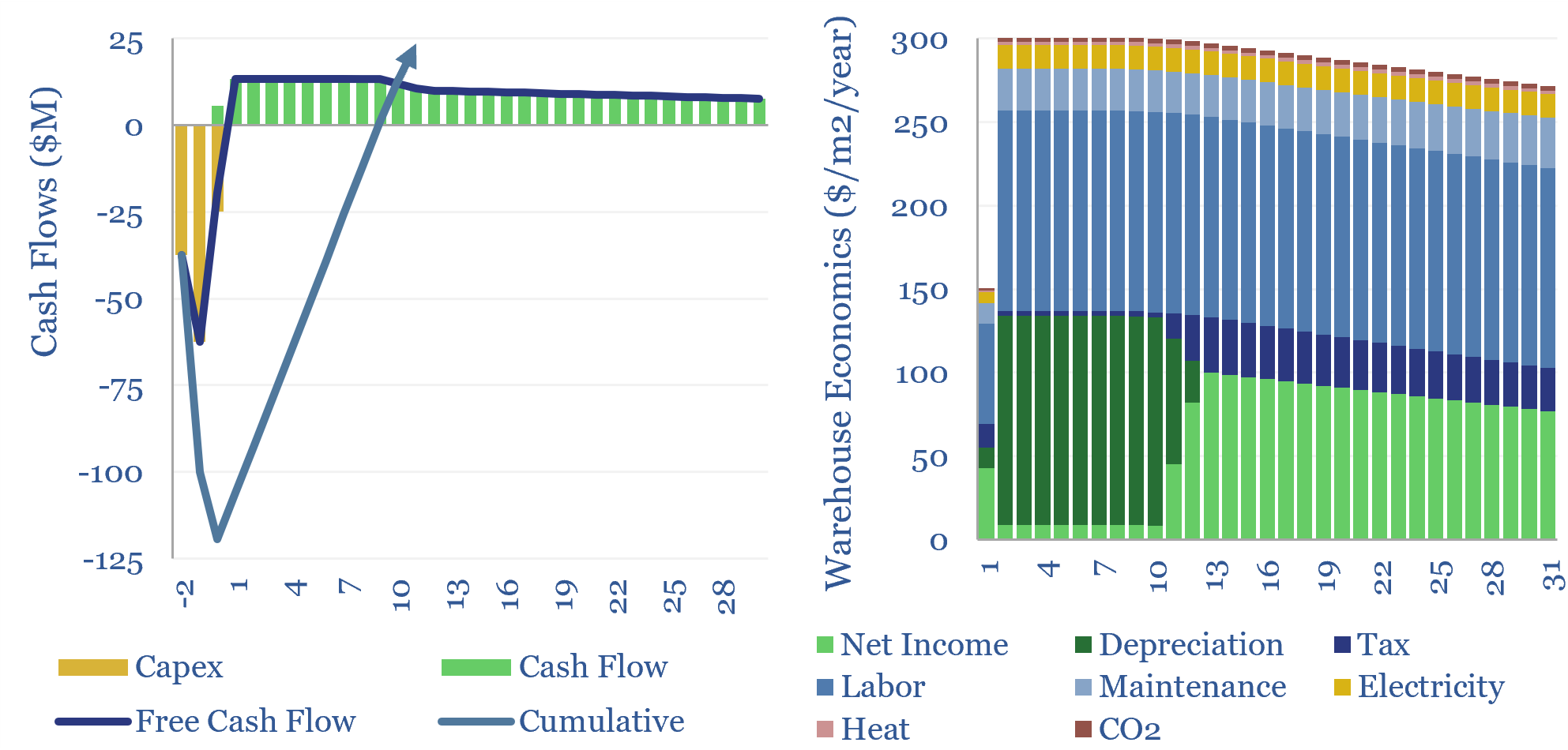
Storage costs: economics of warehouses?

This data-file captures the economics of warehouses. A typical warehousing facility needs to charge $350 per m2 per year of storage, to earn an 8% unlevered return, on $1,250/m2 of construction capex, net of labor, electricity, heating and maintenance costs.
-
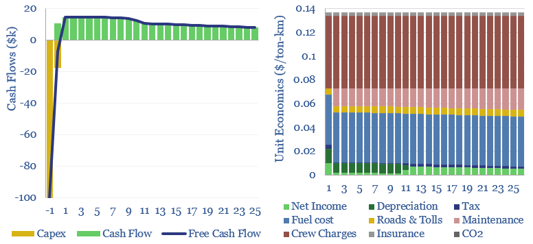
Heavy truck costs: diesel, gas, electric or hydrogen?

Heavy truck costs are estimated at $0.14 per ton-kilometer, for a truck typically carrying 15 tons of load and traversing over 150,000 miles per annum. Today these trucks consume 10Mbpd of diesel and their costs absorb 4% of post-tax incomes. Hydrogen trucks would be 45-75% more costly, but from 2026, we are starting to see…
-
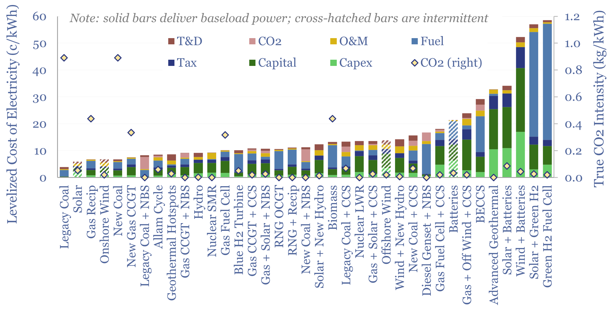
Levelized cost of electricity: stress-testing LCOE?

This data-file summarizes the levelized cost of electricity, across 35 different generation sources, covering 20 different data-fields for each source. Costs of generating electricity can vary from 2-200 c/kWh. The is more variability within categories than between them. Numbers can readily be stress-tested in the data-file.
-
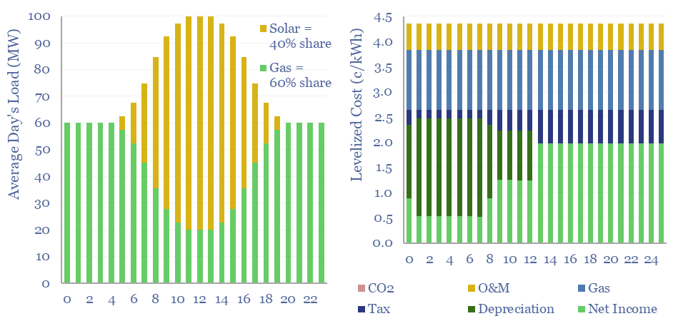
Renewables+gas LCOEs versus standalone gas turbines?

Levelized costs of electricity depend as much on the system being electrified as the energy sources used to electrify it. This data-file captures solar+gas LCOEs (in c/kWh), when meeting different load profiles, as a function of solar capex (in $/kW), gas prices (in $/mcf), and the relative utilization of solar vs gas.
-
US shale gas: the economics?

US shale gas economics are captured in this data-file, requiring a $2.5/mcf hub-level gas price, for a 10% IRR, on a large, $17M shale gas well in a basin such as the Marcellus. The marginal cost for unlocking c3% pa production growth from key shale basins is likely in a range of $3-4/mcf, but the…

Content by Category
- Batteries (96)
- Biofuels (44)
- Carbon Intensity (48)
- CCS (64)
- CO2 Removals (9)
- Coal (41)
- Commentary (65)
- Company Diligence (105)
- Data Models (923)
- Decarbonization (162)
- Demand (130)
- Digital (87)
- Downstream (47)
- Economic Model (221)
- Energy Efficiency (76)
- Hydrogen (63)
- Industry Data (308)
- LNG (56)
- Materials (86)
- Metals (88)
- Midstream (45)
- Natural Gas (161)
- Nature (76)
- Nuclear (28)
- Oil (176)
- Patents (39)
- Plastics (44)
- Power Grids (156)
- Renewables (153)
- Screen (137)
- Semiconductors (35)
- Shale (58)
- Solar (72)
- Supply-Demand (53)
- Vehicles (94)
- Video (24)
- Wind (47)
- Written Research (407)