Natural Gas
-
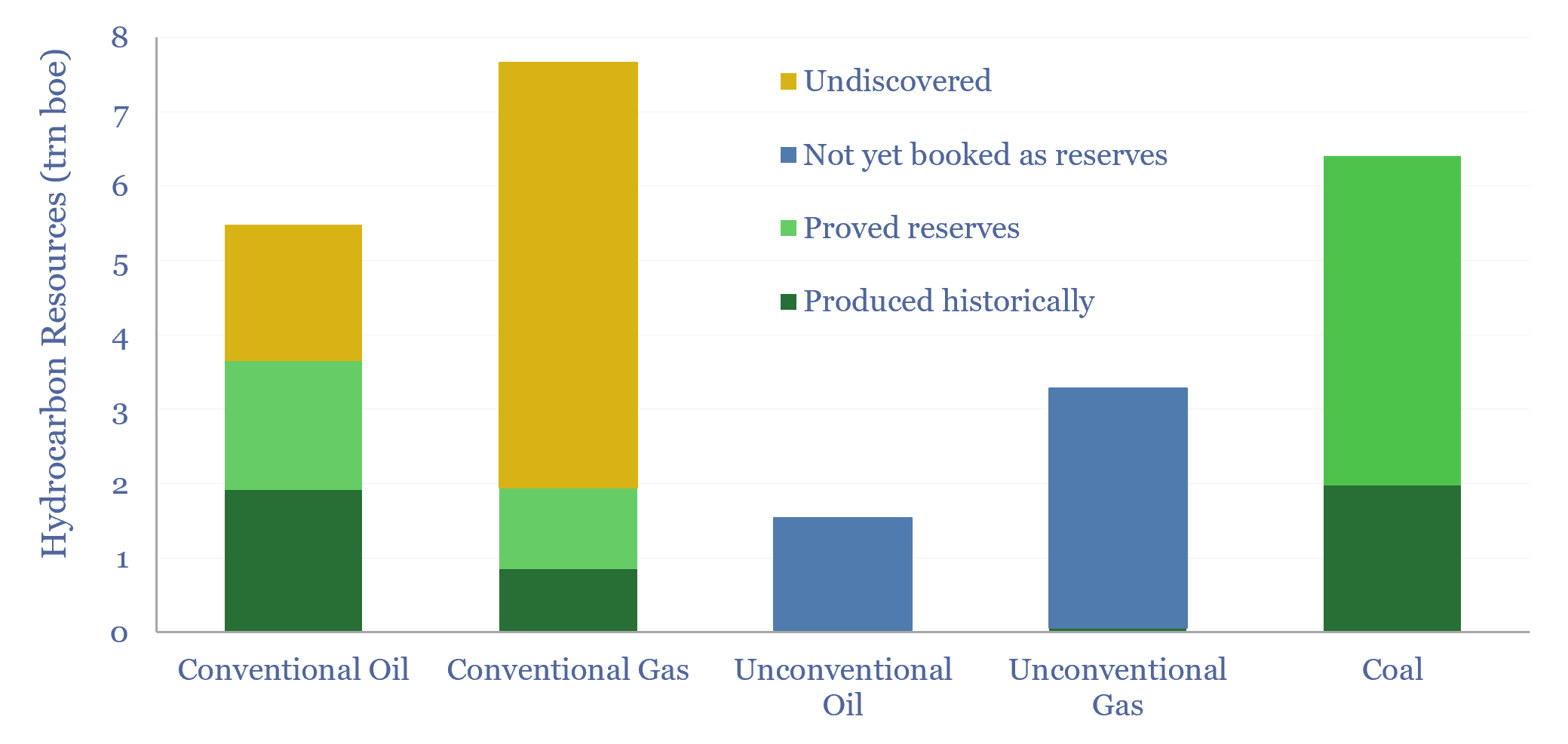
Global hydrocarbon resources: across the history of the world?

We have quantified global hydrocarbon resources, from first principles, in this 15-page report. We estimate how much oil, gas and coal ever formed across the total history of the world. And more importantly, we estimate how much is left. Our numbers support an energy transition from coal to gas.
-
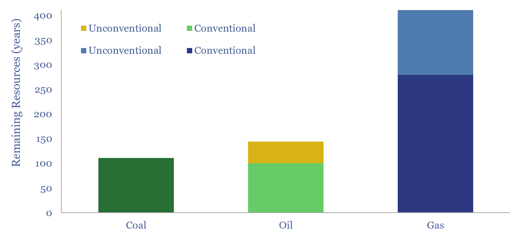
Global hydrocarbon resources and coal resources?

Global hydrocarbon resources and global coal resources — in-place resources and economically recoverable resources — are estimated from first principles in this data-file. We see the world’s remaining economically recoverable reserves of oil and gas being 4x larger than remaining economically recoverable reserves of coal.
-
Global gas supply-demand in energy transition?

Global gas supply-demand is predicted to rise from 400bcfd in 2023 to 650bcfd by 2050, in our outlook, as a complement to wind, solar, nuclear, and as global coal resources mature from the 2030s onwards. This data-file quantifies global gas demand and supply by country, across heating, power and industry.
-
Residential heating costs: boilers, furnaces, electric and heat pumps?
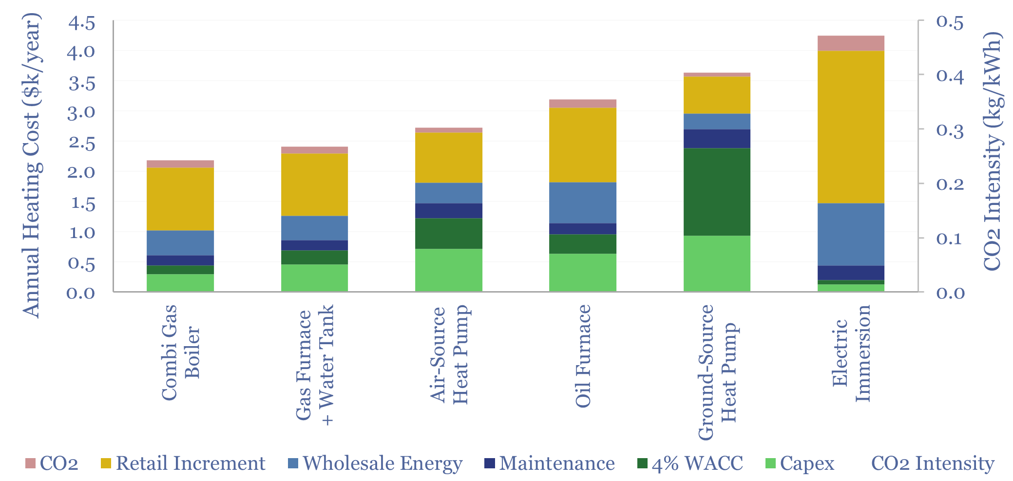
Residential heating costs are compared and contrasted in this data-file, for gas-fired combi boilers, gas furnaces and hot water tanks, oil furnaces and hot water tanks, purely electric heating systems including immersion heaters, air-source heat pumps and ground-source heat pumps. Capex, maintenance and input energy prices can be stress-tested.
-
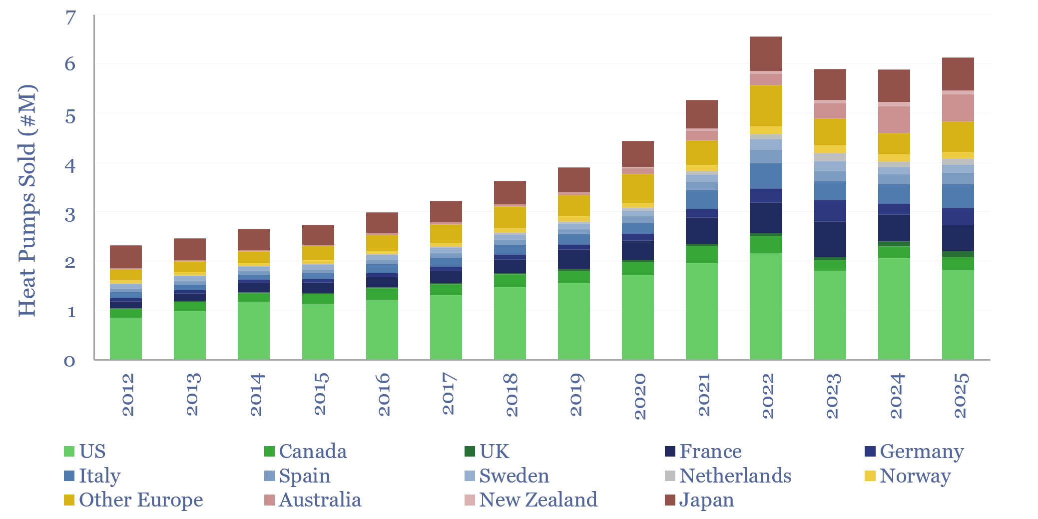
Global heat pump sales by country?

Global heat pump sales by country are tabulated in this data-file, for 14 countries/regions. Developed world heat pump sales rose at an 11% CAGR over the decade since 2012, reaching 6.5M units sold in 2022, but then unexpectedly fell by -10% to 2024. 2025 has seen the start of a recovery, with sales rising 4%…
-
Canadian shale producers and E&P costs?
This data-file is a screen of Canadian upstream companies and Canadian shale producers, especially focused on the fast-growing Montney-Duvernay shale plays. Key themes are rising shale oil and gas production, low-capex wells, high well-level IRRs, performance improvements and consolidation via M&A.
-
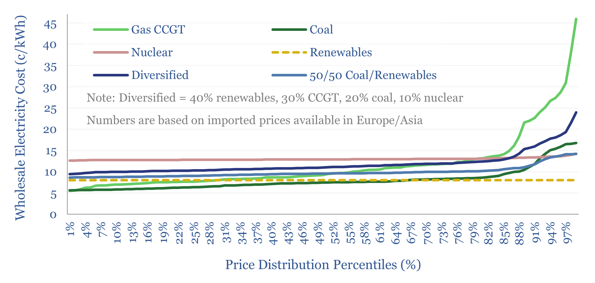
Global power: what grid mix is most stable?

Energy importing countries value stable electricity prices. Hence this 18-page report evaluates the optimal grid mix, after taking stability into account? Recent gas price volatility will encourage further diversification for developed world importers, while coal+solar could dominate emerging world growth. Our forecasts are revised.
-
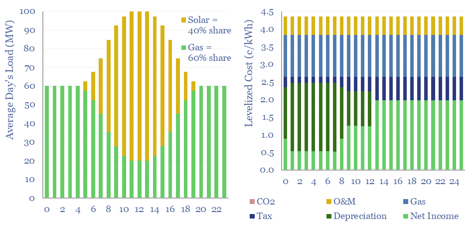
Renewables+gas LCOEs versus standalone gas turbines?

Levelized costs of electricity depend as much on the system being electrified as the energy sources used to electrify it. This data-file captures solar+gas LCOEs (in c/kWh), when meeting different load profiles, as a function of solar capex (in $/kW), gas prices (in $/mcf), and the relative utilization of solar vs gas.
-
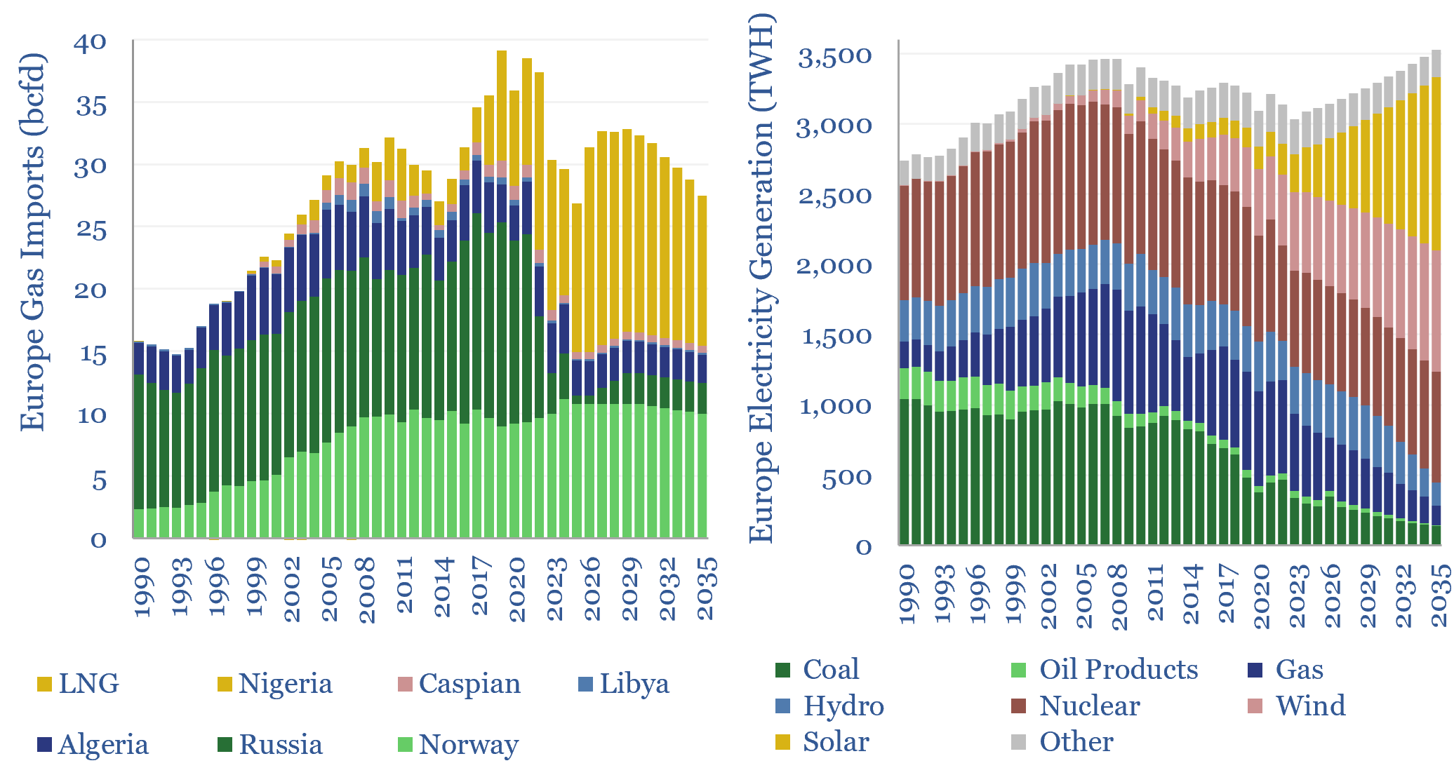
European gas and power model: natural gas supply-demand?

This data-file is our European gas supply-demand model. Balances are assessed in European gas and power markets from 1990 to 2035, reflecting all of our research into Europe’s energy transition. 2024-25 gas markets were supported by inventory draw-downs, but LNG imports step up from 110MTpa to 120MTpa through 2030, before softening again through 2035.
-
US shale gas: the economics?

US shale gas economics are captured in this data-file, requiring a $2.5/mcf hub-level gas price, for a 10% IRR, on a large, $17M shale gas well in a basin such as the Marcellus. The marginal cost for unlocking c3% pa production growth from key shale basins is likely in a range of $3-4/mcf, but the…


Content by Category
- Batteries (96)
- Biofuels (44)
- Carbon Intensity (48)
- CCS (64)
- CO2 Removals (9)
- Coal (44)
- Commentary (65)
- Company Diligence (105)
- Data Models (927)
- Decarbonization (163)
- Demand (131)
- Digital (90)
- Downstream (47)
- Economic Model (222)
- Energy Efficiency (76)
- Hydrogen (63)
- Industry Data (311)
- LNG (56)
- Materials (86)
- Metals (89)
- Midstream (45)
- Natural Gas (163)
- Nature (76)
- Nuclear (28)
- Oil (178)
- Patents (39)
- Plastics (44)
- Power Grids (156)
- Renewables (153)
- Screen (138)
- Semiconductors (35)
- Shale (58)
- Solar (72)
- Supply-Demand (53)
- Vehicles (94)
- Video (24)
- Wind (46)
- Written Research (409)