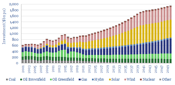
Is the world investing enough in energy?

Global energy investment in 2020-21

Global energy investment in 2020-21 has been running 10% below the level needed on our roadmap to net zero. Under-investment is steepest for solar, wind and gas. Under-appreciated is that each $1 dis-invested from fossil fuels must be replaced with $25 in renewables, to add the same new energy supplies. Future energy capex requirements are staggering. These are the conclusion in our 14-page note.


This 14-page note compares annual energy investment in different upstream energy sources with the amounts that would be required on our roadmap to net zero. The methodology is explained on page 2.

Current investment levels in each energy source are described on pages 3-5, reviewing the trajectory for each major category: oil, gas, coal, wind and solar. A stark contrast is found in capex per MWH of new added energy supplies.

We have constructed 120 different models, in order to stress-test the capex costs per MWH of new added energy supplies, across different resource types. Conclusions and comparisons from our modelling are presented on pages 6-8.

How much would the world need to be investing, on our roadmap to net zero, or indeed on the IEA’s roadmap to net zero? We develop our numbers, category by category, on pages 9-12, to identify where the gaps are greatest.

Conclusions and controversies are laid out on pages 13-14. Disinvestment from oil and gas will tend to exacerbate future energy shortages. To avoid this, it would be ideal to replace each dis-invested $1 of oil and gas investment with around $25 of new renewables investment.

Integrated energy: a new model?

building blocks for a zero-carbon energy

This 14-page note lays out a new model to supply fully carbon-neutral energy to a cluster of commercial and industrial consumers, via an integrated package of renewables, low-carbon gas back-ups and nature based carbon removals. This is remarkable for three reasons: low cost, high stability, and full technical readiness. The prize may be very large.


Four building blocks for a zero-carbon energy mix are outlined on pages 2-5. They include wind, solar, gas-fired CHPs and gas-fired CCGTs. Costs, CO2 intensities and key debates are reviewed for each technology.

Taking out the CO2 requires high-quality nature based carbon removals, for any truly ‘carbon neutral’ energy mix. Meeting this challenge is described on pages 5-7. There will be nay-sayers who do not like this model. To them, we ask, why do you hate nature so much?

Finding a fit requires combining the different building blocks above into an integrated energy system. We find the optimal fit is for renewables capacity to cover 110% of average grid demand. The balancing act is outlined on pages 8-10.

The gas supply chain that backs up the renewables must minimize methane leaks and use the gas as efficiently as possible. Our suggestions are laid out on pages 11-12.

The commercial benefits of this integrated model are described on pages 13-14. We think this is an excellent opportunity to provide fully carbon-neutral energy, using fully mature technologies, at costs well below 10c/kWh and highly bankable price-stability.

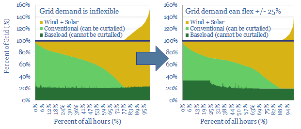
Shifting demand: can renewables reach 50% of grids?

Shifting demand for wind and solar

25% of the power grid could realistically become ‘flexible’, shifting its demand across days, even weeks. This is the lowest cost and most thermodynamically efficient route to fit more wind and solar into power grids. We are upgrading our renewables ceilings from 40% to 50%. This 22-page note outlines the growing opportunity in demand shifting.


Renewables would struggle to reach 50% penetration of today’s grids, due to their volatility. Pages 2-7 quantify the challenges, which include capacity payments for non-renewable back-ups, negative power pricing >20% of the time, >10% curtailment and 30% marginal cost re-inflation for new projects.

But a greater share of renewables would help decarbonization. This objective is explained on page 8, showing the relative costs and CO2-intensities of electricity technologies.

Renewable electricity storage is not the solution. It is costly and thermodynamically inefficient, which actually dilutes the impact of renewables. Costs and efficiency losses are quantified for batteries and for hydrogen on pages 9-11.

Demand shifting is a vastly superior solution. Pages 12-17 outline half-a-dozen demand-shifting opportunities that have been profiled in our research to-date. Companies in the smart energy supply chain are also noted and screened.

What impacts? We model that up to 25% of the grid can ultimately be demand-flexible, while this can help accommodate an additional 10pp share for renewables in the grid, before extreme volatility begins to bite (see pages 18-19).

Europe leads, and we now assume renewables can reach 50% of its power grid by 2050, with follow-through consequences for our gas and power models (page 20).

Our global renewables forecasts are not upgraded, as the bottleneck on a global basis is simply annual capacity additions, which must treble between 2020 and 2050, in our roadmap to ‘net zero’. (pages 21-22).

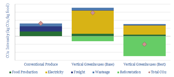
Vertical greenhouses: what future in the transition?

Vertical greenhouses in the energy transition

Vertical greenhouses achieve 10-400x greater yields per acre than field-growing, by stacking layers of plants indoors, and illuminating each layer with LEDs. Economics are exciting. CO2 intensity varies. But it can be carbon-negative in principle. This 17-page case study illustrates how supply chains are localizing and more renewables can be integrated into grids.


The first rationale for vertical greenhouses is to grow food closer to the consumer, which can save 0.6kg of trucking CO2 per kg of food. Eliminating freight is much simpler than decarbonizing freight (pages 2-4).

The second rationale for vertical greenhouses is that they are 10-400x more productive per unit of land, hence they can free up farmland for reforestation projects that absorb CO2 from the atmosphere (pages 5-6).

The third rationale for vertical greenhouses is that their LED lighting demands are flexible, which means they can absorb excess wind and solar, in grids that are increasingly laden with renewables. They are much more economical at achieving this feat than batteries or hydrogen electrolysers (pages 7-10).

The overall CO2 intensity of vertical greenhouses depends on the underlying grid’s CO2 intensity, but the process can in principle become carbon negative (pages 11-13).

Interestingly, we also think vertical greenhouses can smooth our volatile power grids by demand shifting.

The economics are exciting. We model 10% IRRs selling fresh produce at competitive prices, with upside to 30% IRRs if fresher produce earns a premium or operations can be powered with low-cost renewables when the grid is over-saturated (pages 14-15).

Leading companies in vertical greenhouses and in their supply chain are discussed on pages 16-17.

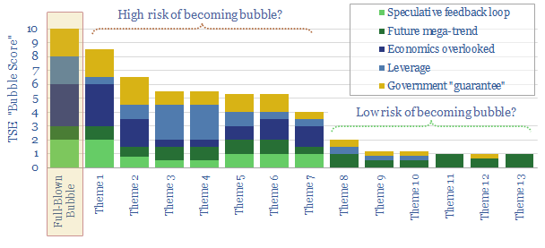
Energy transition: is it becoming a bubble?

Energy transition becoming a bubble?

Investment bubbles in history typically take 4-years to build and 2-years to burst, as asset prices rise c815% then collapse by 75%. In the aftermath, finances and reputations are both destroyed. There is now a frightening resemblance between energy transition technologies and prior investment bubbles. This 19-page note aims to pinpoint the risks and help you defray them.


Our rationale for comparing energy transition to prior investment bubbles is contextualized on page 2, based on discussions we have had with investors and companies in 2020.

Half-a-dozen historical bubbles are summarized on pages 3-4, in order to compare the energy transition with features of Dutch tulips, the South Sea and Mississippi Companies, British Railway Mania, Roaring Twenties, Dot Com bubble and sub-prime mortgages.

Five common features of all bubbles are considered in turn on pages 5-16. In each case, we explain how the feature contributed to past bubbles, and where there is evidence of the feature in different energy transition technologies.

Important findings are that many themes of the energy transition can achieve continued deflation or profitability, but not both; while a combination of increasing leverage and curtailment on renewables assets could leave many assets underwater.

Implications are drawn out on pages 17-19, including five recommendations for decision-makers to find opportunities and avoid the most dangerous aspects of bubbles surrounding the energy transition.

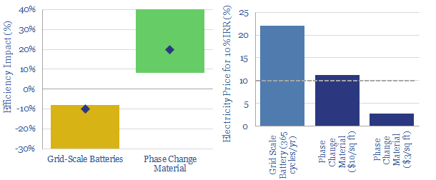
Backstopping renewables: cold storage beats battery storage?

Phase change materials for backstopping renewables

Phase change materials could be a game-changer for energy storage. They absorb (and release) coldness when they freeze (and melt). They can earn double digit IRRs unlocking c20% efficiency gains in freezers and refrigerators, which make up 9% of US electricity. This is superior to batteries which add costs and incur 8-30% efficiency losses. We review 5,800 patents and identify early-stage companies geared to the theme in our new 14-page note.


Refrigerators and freezers comprise 9% of the US electric grid, of which half is in the commercial sector, across 4,200 warehouses, 40,000 supermarkets and 620,000 restaurants. This report argues that a new class of materials, Phase Change Materials (PCMs), can effectively store excess renewable energy as coldness in these fridges and freezers (aka “demand shifting“), improving their efficiency by c20% and without requiring power prices to increase.

The energy economics of cold storage are explained on pages 2-4, outlining the energy consumption of cold storage facilities as function of different input variables (which will also help you understand how to save energy at your fridge-freezer at home) .

Phase change materials are explained on pages 5-6, explaining what they are, how they work, and how they can lower energy consumption by c20% at a typical fridge/freezer.

The economics are modelled on pages 7-8, showing an 8.5% IRR under recent costs and power prices, rising into double digits with a CO2 price, and above 30% with recent deflation in the costs of PCMs.

A comparison with battery storage is provided on page 9-10, showing a clear preference for PCMs. Batteries decrease efficiency and raise electricity costs. PCMs increase efficiency and do not raise electricity costs. Batteries have further challenges.

Who are the leading companies commercialising PCMs? We answer this question on pages 11-14, by reviewing 5,800 patents. We find promising venture-stage and growth-stage companies in the space, plus listed companies in the capital goods, materials and automotive sectors.

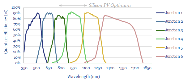
Solar energy: is 50% efficiency now attainable?

solar efficiency in record-breaking multi-junction cells

Most commercial solar cells achieve 15-25% efficiencies, converting incoming solar energy into usable electricity. But a new record has been published in 2020, achieving 47.1% conversion efficiency. The paper used “a monolithic, series-connected, six-junction inverted metamorphic structure under 143 suns concentration”. Our goal in this short note is to explain this solar efficiency record.


“A monolithic, series-connected, six-junction inverted metamorphic structure under 143 suns concentration”

p-n junctions are the foundation of all solar cells. Each side of the junction is doped, so that the “n”-side will surrender electrons, while the “p”-side will accept electrons. When incoming solar energy strikes the junction, it may dislodge an electron and leave behind a hole. The liberated electron will propagate towards the “p”-side, while the holes will propagate towards the “n”-side, thus creating a direct current.

Bandgap is the energy needed to dislodge an electron from its usual orbit, so it is free to move through a p-n junction. The energy in light varies with wavelength (lower-wavelength equals lower energy). Light waves below the bandgap will not suffice to dislodge electrons: they will pass through the material and the energy will not be captured. Light waves above the bandgap will have excess energy left over after dislodging electrons: the excess energy will be lost as heat.

Single-junction solar cells are composed of p-n junctions made of a single material, most commonly crystalline silicon, in today’s commercial solar industry. Silicon atoms have a bandgap of 1.4eV and achieve optimum conversion efficiency in light with 700-1,000nm wavelengths (red and infra-red). They do not capture energy efficiently from lower energy, lower wavelength light (such as 400-700nm) or very high wavelength light (1,000nm+).

Multi-Junction solar cells aim to overcome the limitations of single-junction solar cells, combining multiple p-n junctions, made of multiple solar materials, to capture a broader range of the spectrum. For example, the six-junction solar cell discussed in this note has six separate junctions, connected in series, to capture light from c350-1700nm wavelengths, which is tantamount to c65-85% of all the energy in sunlight.

Group III-V alloys are used in different combinations in each of these junctions, to tune its bandgap, to capture a different wavelength of light. These alloys are composed of elements from Groups III and V in the periodic table. Group III includes boron, aluminium, gallium and indium. Group V includes nitrogen, phosphorus, arsenic and antimony.

The junctions are usually stacked with the highest energy absorber on top (i.e., junction 6). Photons that lack sufficient energy to dislodged electrons in junction 6 will pass through it, and have a additional chances of being absorbed in junction 5, through to junction 1.

The challenge is how to stack these six junctions on top of each other in a way that limits recombination and resistance, both of which are going to impair solar cell efficiency.

The challenge of recombination?

Recombination occurs when dislodged electron and holes re-combine in a solar cell, thereby lowering the current reaching the current collectors. If recombination re-emits photons, it is known as radiative recombination. Group III-V solar cells are particularly sensitive to recombination around dislocations.

Dislocations are abrupt changes in the crystal structures in a material. A physical effect is that dislocations allow atoms to glide or slip past one another at low stress levels. An optoelectronic effect is to impede current and encourage recombination of electrons and holes.

One type of dislocation, known as a threading dislocation because of its shape, extends beyond the surface of the strained layer and throughout the material, so it can be particularly deleterious to solar cell performance.

Multi-junction solar cells are particularly prone to dislocations because each junction is made of a different material. These materials are lattice-mismatched monoliths.

Monolithic materials are formed a single, continuous and unbroken crystal structure, all the way to its edges, with minimal defects or grain boundaries. This means it does not suffer from grain boundaries or dislocations, and in turn, efficiency losses from recombination should be minimized. But it is very difficult to manufacture monolithic materials from lattice-mismatched components.

Lattice-mismatched materials have different lattice constants. This means that they are composed of crystals of different sizes. In turn, this means they will not adhere well to one-another. Their boundaries are prone dislocations.

The solution: metamorphic epitaxy?

A technique called metamorphic epitaxy was used to create the monolithic six-junction solar cells described above, and overcome the inter-related challenges of recobination at dislocations in lattice mismatched materials.

Epitaxy is the process of orientation-controlled growth of crystals on top of other crystals. The 47% efficient solar cell used a variant called organometallic vapour phase epitaxy (OMVPE). Our overview of manufacturing methods is here.

Metamorphic epitaxy minimizes dislocations around the active site of an engineered material. This is achieved by relieving the strain around lattice-mismatched boundaries by encouraging dislocations to occur away from the active site of the material. Specifically, materials known as Compositionally Graded Buffers (CGBs) were introduced in between the fourth to sixth junctions of the six-junction solar cell, as thse were the boundaries most prone to dislocations.

Specifically, these six-junction solar cells were monolithically grown on a single 2×3 cm GaAs substrate, at 550-750C temperatures, in an atmospheric-pressure OMVPE system.  “Growth begins with the high-bandgap lattice-matched junctions [on the bottom], leaving these high-power-producing junctions without dislocations”.

Then the cell was then inverted as the high bandgap lattices need to be situated on the top of the cell. (In other words, the cell is printed upside down and then turned over). Gold was electroplated onto contact of the inverted structure (literally, “gold-plated”!), then the cell was epoxied onto a flat silicon wafer. The GaAs substrate was removed by chemical etching. A front-side grid of NiAu was deposited by photolithography. Finally an anti-reflective coating of MgF2/ZnS/MgF2/ZnS was thermally deposited on the top of the cell.

The full 6J IMM structure consisted of 140 layers, including individual compositional step-graded buffer layers. The total growth time was 7.5 h.

1 sun’s concentration?

Under 1 sun’s solar intensity, the cell described above achieved 39.2% efficiency. This is the highest 1-Sun conversion efficiency demonstrated by any technology to-date. The prior record is 38.8% for a five-junction bonded III–V solar cell.

The efficiency is very high, because the voltages of each junction add up to a high total voltage. However, the current density in each junction was low. The efficiency could have been higher with a higher current density, which in turn, is achieved by concentrating the incoming sunlight.

143 suns’ concentration?

Concentration of incident light improves solar cell efficiency. The reason is that more concentrated light dislodges more electrons. More dislodged electrons means a higher current density. In turn, a higher current density raises the bandgap for dislodging further electrons (it is harder to remove further electrons from a material that has already lost some electrons). So even more energy can be absorbed when additional light strikes the cell.

Concentrating solar light is also desirable as a way to lower costs, as multi-junction solar cells are expensive to produce. Concentrating the light from 1 square meter onto 1 square centimeter, for example, reduces the area of solar materials required by a factor of 10,000.

Joule losses set the upper limit on the solar concentration that will maximize efficiency. Joule losses are the loss of electricity as heat when electric current passes through a conductor. They are a square function of current and a linear function of resistance. So they rise quadratically as solar intensity rises linearly.

Lower resistance will help to limit joule losses. In the solar cell described above, several challenges were observed keeping resistance low.

Each junction is connected in series in the cell. The current flows between each junction through a “tunnel interconnection”. Resistance through these tunnel junctions was found to rise with current, placing a practical limit on solar concentrations.

Internal resistances within each junction were also higher than desired. They were found to have been elevated by the temperatures during epitaxy and during dopant diffusion (particularly in Zn-containing layers).

At the top junction, the 2.1eV bandgap material required a high resistance to conduct charge laterally to the metal grid fingers that serve as current collectors for the cell’s electrical circuit.

Reducing the effective series resistance to 0.015 Ω cm2 is seen to be possible, by analogy to previous four-junction solar cells, which would allow the six-junction cell described above to surpass 50% efficiency at 1,000–2,000 Suns. The maximum theoretical efficiency is 62%.

Commercial implications?

47-50% efficient solar cells are a good incremental improvement. To put the ‘breakthrough’ into context, the previous record for a multi-junction solar cell was 46% efficiency at 508 suns, using a four-junction device. There is scope for multi-junction solar cell efficiency to improve further.

The cell was also very small, at 0.1cm2. When solar ‘records’ are measured, usually the stipulation is required that a cell must be 1cm2 in area, as a testing criterion.

Its production was very complex taking 7.5-hours to assemble 140 separate layers. Complex structures are expensive and more prone to degradation, which makes commerciality challenging.

We conclude that a 47-50% efficient solar cell is a tremendous technical achievement. But the evidence does not yet suggest proximity to commercialising ultra-efficient multi-junction solar cells like this at mass scale. All of our solar research is summarized here.


Source: Geisz, J. F., France, R. M., Schulte, K. L., Steiner, M. A., Norman, A. G., Guthrey, H. L., Young, M. R., Song, T. & Moriarty, T. (2020). Six-junction III–V solar cells with 47.1% conversion efficiency under 143 Suns concentration. National Renewable Energy Laboratory (NREL), Golden, CO, USA.

Ten Themes for Energy in the 2020s

We presented our ‘Top Ten Themes for Energy in the 2020s’ to an audience at Yale SOM, in February-2020. The audio recording is available below. The slides are available to TSE clients, in order to follow along with the presentation.


Please sign up to our distribution list, to receive our best ideas going forwards…

=

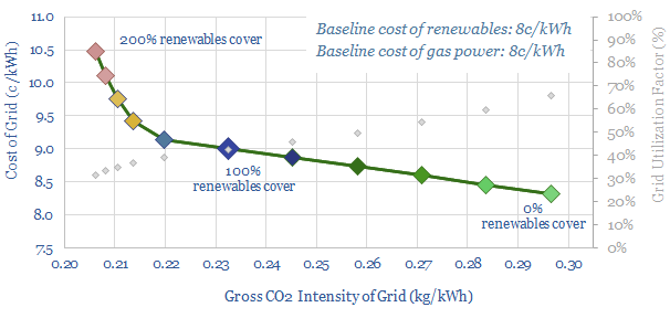
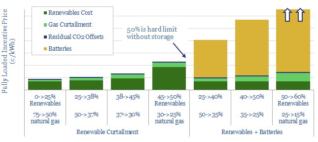
Decarbonized power: how much wind and solar fit the optimal grid?

when will wind and solar peak?

What should future power grids look like? Our 24-page note optimizes cost, resiliency and CO2, using a Monte Carlo model. Renewables should not surpass 45-50%. By this point, over 70% of new wind and solar will fail to dispatch, while incentive prices will have trebled. Batteries help little. They raise power prices by a further 2-5x to accommodate just 3-15% more renewables. The lowest-cost, zero-carbon power grid, we find, comprises c25% renewables, c25% nuclear and c50% decarbonized gas, with an incentive price of 9c/kWh.


Pages 2-4 illustrate the volatility of wind and solar generation at today’s grid penetration, providing rules of thumb around intermittency.

Pages 5-6 illustrate the strange consequences once renewables surpass 25% of the grid, including curtailment, negative power pricing and financing difficulties.

Pages 7-9 quantify and explain how much curtailment will take place in a typical grid as renewables scale from 25% to 40%, 50% and 60% of gross generation, using a Monte Carlo approach. The model shows when and why curtailment is occurring.

Pages 10-20 quantify and explain the costs of batteries, to backstop renewables as they scale from 25%, to 40%, 50% and 60% of the grid, while avoiding curtailment. Real world conditions are not conducive to competitive battery economics.

Pages 21-23 quantify the residual reliance on natural gas. Amazingly, even our most aggressive battery scenarios only permit 10% of gas-power capacity to be shuttered. Low-utilization gas is costly. High-utilization gas is less costly. And the economics of decarbonized gas are superior to any renewables plus batteries combination.

Page 24 concludes that natural gas will emerge as the ‘best battery’ to backstop renewables, estimating the most likely shares in an optimal power mix.

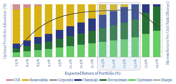
Ramp Renewables? Portfolio Perspectives.

optimal portfolios transitioning to renewables.

It is often said that Oil Majors should become Energy Majors by transitioning to renewables. But what is the best balance based on portfolio theory? Our 7-page note answers this question, by constructing a mean-variance optimisation model. We find a c0-20% weighting to renewables maximises risk-adjusted returns. The best balance is 5-13%. But beyond a c35% allocation, both returns and risk-adjusted returns decline rapidly.


Pages 2-3 outline our methodology for assessing the optimal risk-adjusted returns of a Major energy company’s portfolio, including the risk, return and correlations of traditional investment options: upstream, downstream and chemicals.

Page 4 quantifies the lower returns that are likely to be achieved on renewable investment options, such as wind, solar and CCS, based on our recent modeling.

Pages 5-6 present an “efficient frontier” of portfolio allocations, balanced between traditional investment options and renewables, with different risk and return profiles.

Pages 6-7 draw conclusions about the optimal portfolios, showing how to maximise returns, minimise risk and maximise risk-adjusted returns (Sharpe ratio).

The work suggests oil companies should primarily remain oil companies, working hard to improve the efficiency and lower the CO2-intensities of their base businesses.

Copyright: Thunder Said Energy, 2019-2024.