-
Delivery drones: flight trajectory?

Delivery drones are finally taking off? Pilot projects in the US are achieving strong safety records, exciting consumers and raising the prospect of sub-$1 deliveries within 10-minutes. This 13-page report explores the future impacts of delivery drones in energy, materials and capital goods.
-
Capital goods: book-to-bill ratio tracker?

How long will boom times last in capital goods categories, including for AI data center construction? To answer this question, we have started tracking book-to-bill ratios, across 40 capital goods categories, from companies quarterly results. Booms occur when book-to-bill exceeds 1.5x, and typically last 2-years.
-
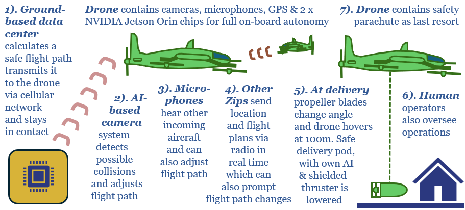
Zipline: drone delivery technology?

Details of Zipline drone delivery technology are derived in this data-file, based on reviewing over 15 highly detailed patent families from the company. We see a moat around specific hardware innovations, a low cost sensor suite, inherent safety from seven layers of safety protections, and a sophisticated fleet management system.
-
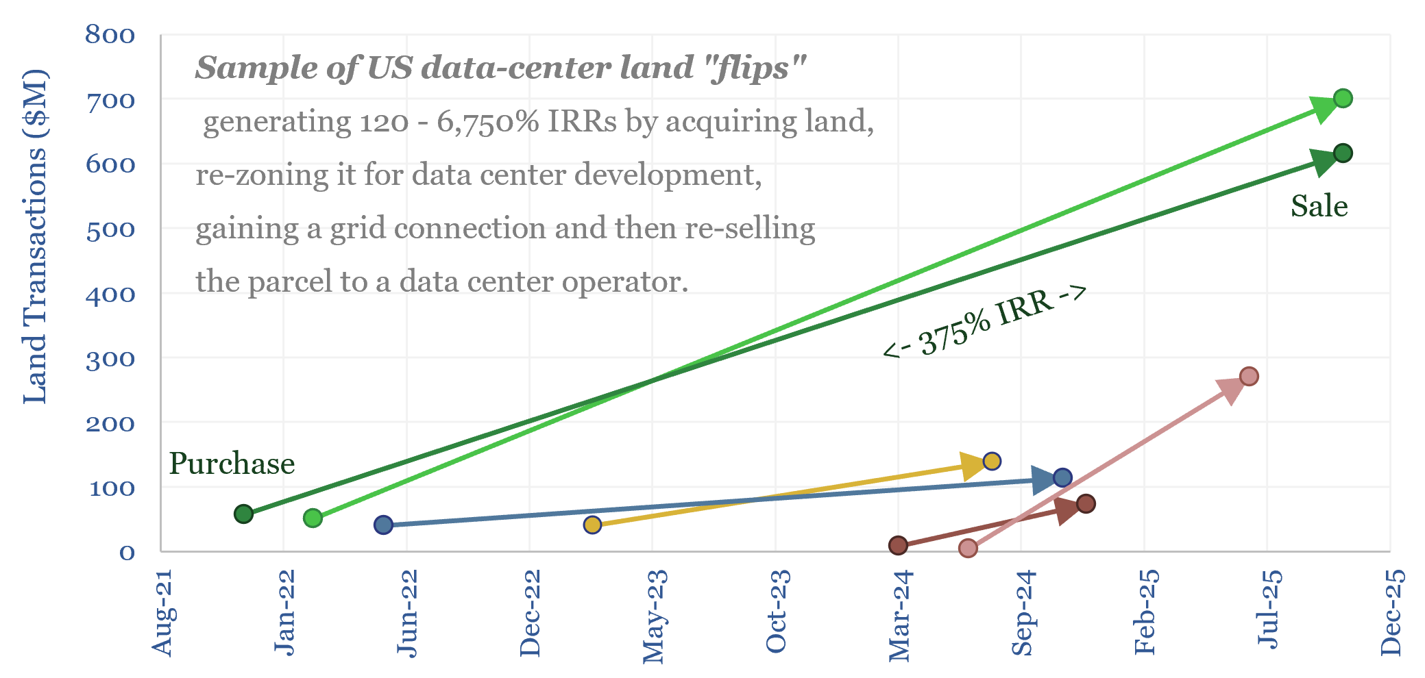
Electrical service agreements: how real are those data centers?
Are speculative data center projects, 80% of which will never get built, inflating future load growth forecasts? This 18-page report reviews evidence from land developer returns, recent PUC deliberations and evolving terms in Electrical Service Agreements (ESAs).
-
Energy economics: an overview?
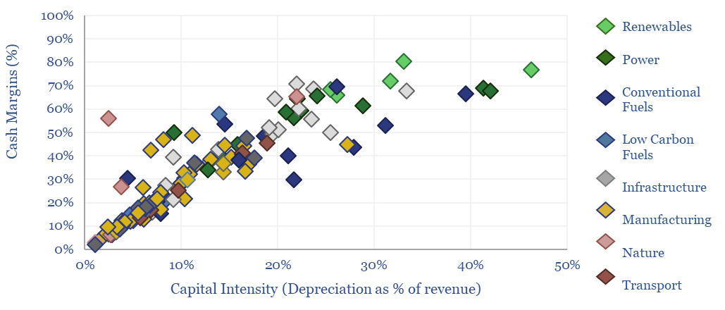
This data-file provides an overview of energy economics, across 175 different economic models constructed by Thunder Said Energy, in order to put numbers in context. This helps to compare marginal costs, capex costs, energy intensity, interest rate sensitivity, and other key parameters that matter in the energy transition.
-
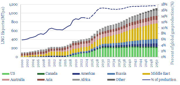
LNG: top conclusions in the energy transition?

Thunder Said Energy is a research firm focused on economic opportunities that drive the energy transition. Our top ten conclusions into LNG are summarized below, looking across all of our research.
-
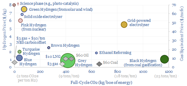
Hydrogen: overview and conclusions?

We think the best opportunities in hydrogen will be to decarbonize gas at source via blue and turquoise hydrogen, displacing ‘black hydrogen’ that currently comes from coal, and to produce small-scale feedstock on site via electrolysis for select industries. Others see green hydrogen as a cornerstone of the future energy system. We think there may…
-
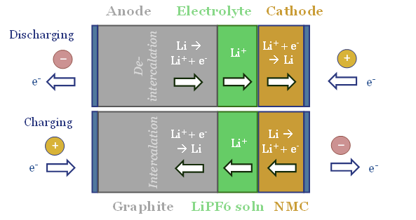
Energy storage: top conclusions into batteries?

Thunder Said Energy is a research firm focused on economic opportunities that can drive the energy transition. Our top ten conclusions into batteries and energy storage are summarized below, looking across all of our research.
-
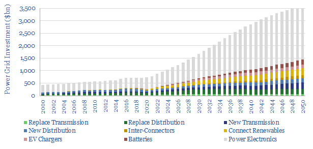
Power grids: opportunities in the energy transition?

Power grids move electricity from the point of generation to the point of use, while aiming to maximize the power quality, minimize costs and minimize losses. Broadly defined, global power grids and power electronics investment must step up 5x in the energy transition, from a $750bn pa market to over $3.5trn pa. But this theme…
-
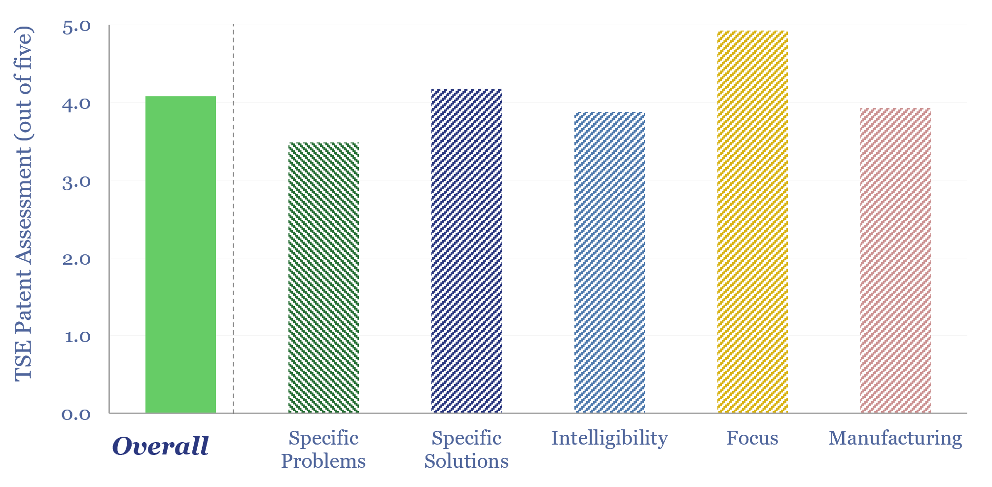
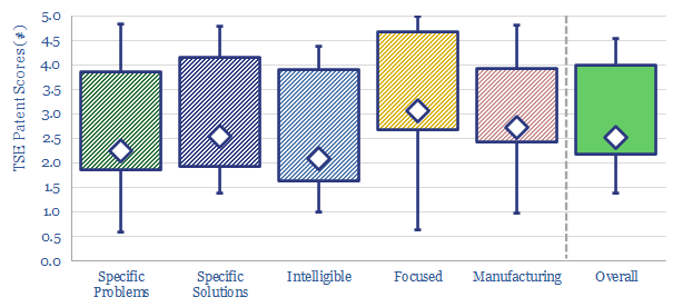
TSE Patent Assessments: a summary?

This data-file aggregates all of our patent assessments into a single reference file, so different companies’ scores can be compared and contrasted. Our average score is 3.5 out of 5.0. Skew is to the downside. Intelligibility is the biggest challenge. Scores correlate with TRL and revenues.
Content by Category
- Batteries (96)
- Biofuels (44)
- Carbon Intensity (48)
- CCS (64)
- CO2 Removals (9)
- Coal (41)
- Commentary (65)
- Company Diligence (105)
- Data Models (924)
- Decarbonization (162)
- Demand (131)
- Digital (88)
- Downstream (47)
- Economic Model (221)
- Energy Efficiency (76)
- Hydrogen (63)
- Industry Data (308)
- LNG (56)
- Materials (86)
- Metals (88)
- Midstream (45)
- Natural Gas (161)
- Nature (76)
- Nuclear (28)
- Oil (176)
- Patents (39)
- Plastics (44)
- Power Grids (156)
- Renewables (153)
- Screen (138)
- Semiconductors (35)
- Shale (58)
- Solar (72)
- Supply-Demand (53)
- Vehicles (94)
- Video (24)
- Wind (47)
- Written Research (408)