This data-file evaluates transmission and distribution costs, averaging 7c/kWh in 2024, based on granular disclosures for 200 regulated US electric utilities, which sell 65% of the US’s total electricity to 110M residential and commercial customers. Costs have doubled since 2005. Which utilities have rising rate bases and efficiently low opex?
Regulated electrical utilities in the US are required to submit their capex, opex and SG&A costs to FERC via Form 1 filings. The data are used to determine acceptable utility charges, and also made freely available to the public, after a lag.
Costs of transmission and distribution utilities have doubled in the past 20-years, even in real terms, from 3.5 c/kWh in 2004-05 to 7c/kWh in 2024. Rising costs would seem to incentivize self-generating, especially amidst grid bottlenecks?
The largest reason for rising costs is rising transmission and distribution capex to accomodate renewables, trebling from 1c/kWh to 3c/kWh. Our numbers actually understate the costs charged to consumers, which will also include a statutory return on prior period capex, in addition to the direct costs that are tabulated in the file. This underscores a conclusion in our recent research: while renewables are a good, low-cost way of decarbonizing, they do add costs on a total system basis.
Over the past ten years, we estimate that 50% of utilities’ direct costs are capex and 50% are opex. The capex is 50% distribution, 35% transmission and 15% plant. The opex is 60% customer G&A, 25% T&D opex and c15% T&D maintenance.
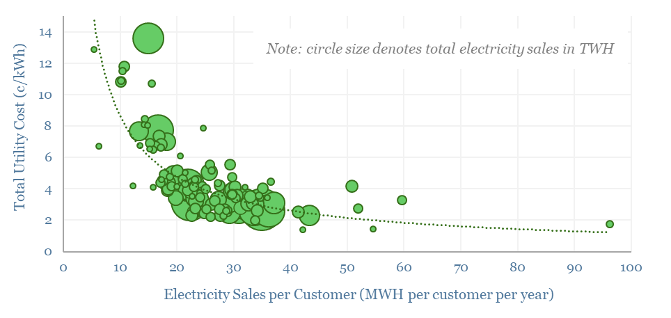
Costs are -60% correlated with average power sales per customer, or in other words, customer type. Across the US, the average residential household uses 10MWH pa, the average commercial business uses 70MWH and the average industrial facility uses 2GWH. Costs approximately halve when average power use per customer doubles.
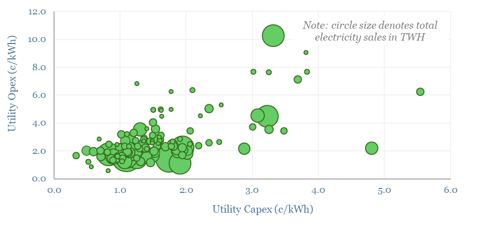
The largest US utilities, with 2-5M customers each and 80-120 TWH pa of electricity sales include PG&E, SCE, FPL, Oncor, ConEd, ComEd, Duke, Centerpoint, DTE. Capex costs range from 0.5-5 c/kWh and opex costs range from 1-10 c/kWh.
The ideal mix is high capex and low opex, as this indicates a well-run utility with a rising rate base and thus rising earnings potential? PSEG, SCE, ConEd, FPL perhaps stand out most on these metrics.
Regulated utilities are not really meant to have pricing power. But bottlenecks are biting, and we do wonder whether value inevitably trickles back to infrastructure owners and operators, in power grids and especially in gas pipelines.
The key drawback to the data that are tabulated in this file is their recency. FERC has released data from 1994-2019 in Excel format, utility by utility. The FERC website has data through 1H21 in dbf format. We will update this data-file if and when further data are made available by FERC.
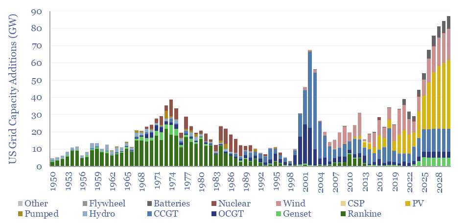
The power demands of AI will contribute to the largest growth of new generation capacity in history. This 18-page note evaluates the power implications of AI data-centers. Reliability is crucial. Gas demand grows. Annual sales of CCGTs and back-up gensets in the US both rise by 2.5x?
Cummins is a power technology company, listed in the US, specializing in diesel engines, underlying components, exhaust-gas after-treatment, diesel power generation and pivoting towards hydrogen. We reviewed 80 patents from 2023-24. What outlook for Cummins technology and verticals in the energy transition?
Hence we have been exploring companies in medium-scale commercial and industrial power generation, such as Generac.
Cummins was founded in 1919, headquartered in Indiana, with 75,500 employees and is listed on NYSE with c$40bn of market cap in 2024.
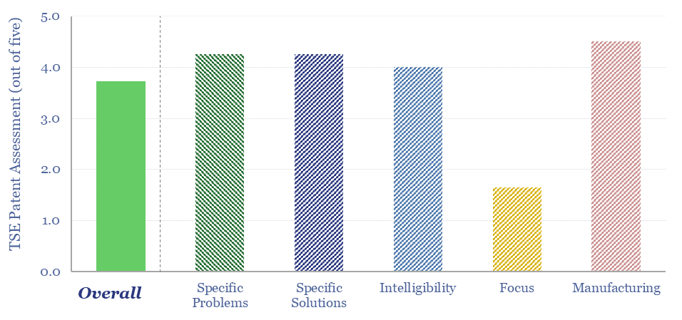
Cummins has filed c5,000 patents historically. We reviewed 80 of the most recent patents filed in 2023-24. Most are clear, articulate specific issues that need to be addressed, including lower-cost or easier manufacturing, then describe specific components and solutions alongside detailed engineering diagrams.
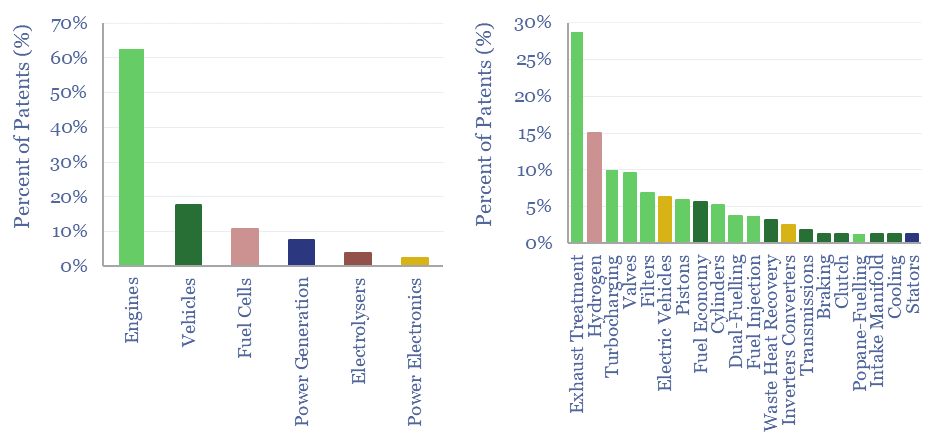
The breakdown of Cummins’s business, by revenue, EBITDA and patent filing focus surprised us, with lower exposure to power generation and a growing focus upon hydrogen.
Based on patent filings, it may even seem as though power generation is being de-prioritized, while hydrogen is being heavily re-prioritized and comprised c15% of recent patents in 2023-24 (chart below).
However the largest focus area remains its core business of diesel engines and exhaust-gas after-treatment (to remove NOx). Our long-term oil demand outlook does see growing demand in this end market.
Exhaust from a diesel engine contains NOx and particulates. An after-treatment unit typically reduces NOx into N2 and H2O using a 30-35% solution of urea in 65-70% deionized water. Heated urea decomposes: CO(NH2)2 + H2O -> 2NH3 + CO2. NH3 then reacts with NO: 4NH3 + 4NO + O2 -> 4N2 + 6H2O. The urea solution is marketed under brands such as AdBlue from BASF. Cummins is among the largest vendors of after-treatment systems in the world, worth >$5bn pa in sales.
However, this business is casting off the shadow of a $1.7bn Clean Air Act fine in 2023, for installing defeat devices. Yet we did find clear, specific and detailed patents improving after-treatment systems.
Another large component of the patents focuses upon diesel engines, improving the fuel economy and resiliency of engines, valves, pistons, cylinders and other components. Details are in the data-file.
This data-file contains our conclusions into Cummins’s diesel engine and generator technology, a broader outlook for some of the company’s verticals, and some undiplomatic comments which we should probably have left out.
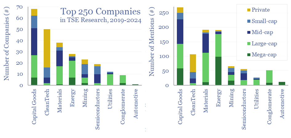
This note summarizes the key conclusions from our energy transition research in 1Q24 and across 1,400 companies in total. Volatility is rising. Power grids are bottlenecked. Hence what stands out in capital goods, clean-tech, solar, gas value chains and materials? And what is most overlooked?
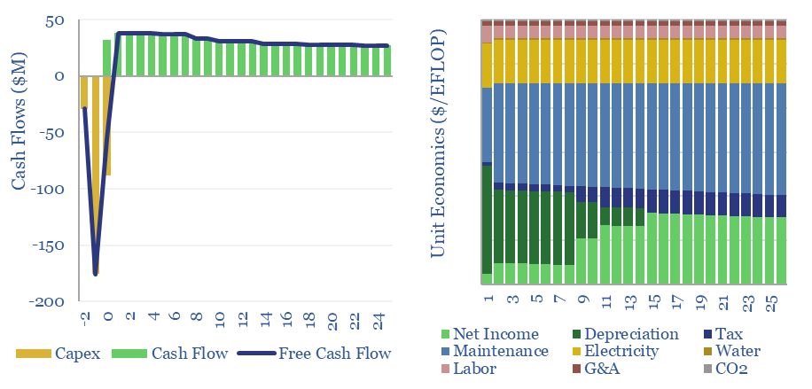
The capex costs of data-centers are typically $10M/MW, with opex costs dominated by maintenance (c40%), electricity (c15-25%), labor, water, G&A and other. A 30MW data-center must generate $100M of revenues for a 10% IRR, while an AI data-center in 2024 may need to charge $3M/EFLOP of compute.
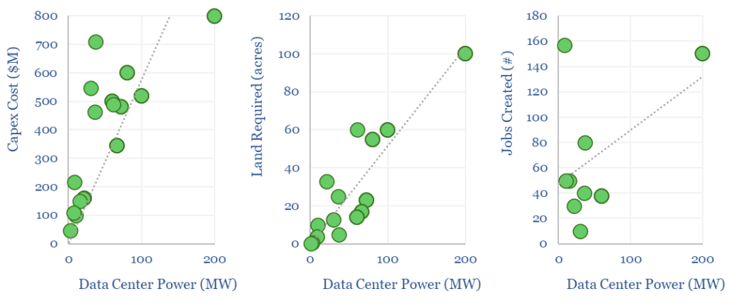
Data-centers underpin the rise of the internet and the rise of AI, hence this model captures the costs of data-centers, from first principles, across capex, opex, land use and other input variables (see below).
In 2023, the global data-center industry is $250bn, across 500 large facilities, 20,000 total facilities, and around 40 GW of capacity, which likely rises by 2-5x by 2030.
A 30MW mid-scale data-center, costing $10M/MW of capex, must generate $100M pa of revenues, in order to earn a 10% IRR, after deducting electricity costs and maintenance.
If the data-center is computation heavy, e.g., for AI applications, this might equate to a cost of around $3/EFLOP of compute in 2023. This fits with disclosures from OpenAI, stating that training GPT 4 had a total compute of 60M EFLOPs and a training cost of around $160M.
However, new generations of chips from NVIDIA will increase the proportionate hardware costs and may lower the proportionate energy costs (see ComputePerformance tab).
Reliability is also crucial to the economics of data-centers: uptime and utilization have a 5x higher impact on overall economics than electricity prices. This makes it less likely that AI data-centers will be demand-flexed to power them using the raw output from renewable electricity sources, such as wind and solar?
Economic considerations may tip the market towards sourcing the most reliably power possible, especially amidst grid bottlenecks, and it also explains the routine use of backup power generation.
Another major theme is the growing power density per rack, rising from 4-10kW to >100kW, and requiring closed-loop liquid cooling.
Please download the data-file to stress-test the costs of a data-center, performance of an AI data-center, and we will also continue adding to this model over time. Notes from recent technical papers are in the final tab.
What if large quantities of power could be transmitted via the 2-6 GHz microwave spectrum, rather than across bottlenecked cables and wires? This 12-page note explores the technology, advantages, opportunities, challenges, efficiencies and costs. We still fear power grid bottlenecks.
Electromagnetic radiation is a form of energy, exemplified by light, infrared, ultraviolet, microwaves and radio waves. What is the energy content of light? How much of it can be captured in a solar module? And what implications? We answer these questions by modelling the Planck Equation and Shockley-Queisser limit from first principles.
Electromagnetic radiation is the synchronized, energy-carrying oscillation of electric and magnetic fields, which moves through a vacuum at the speed of light, which is 300,000 km per second.
Most familiar is visible light, with wavelengths of 400 nm (violet) to 700 nm (red), equating to frequencies of 430 (red) to 750 THz (violet).
At the center of the solar system, our sun happens to emit c40% of its energy in the visible spectrum, 50% as infra-red and c10% as ultraviolet, and very little else (e.g., X-rays, gamma rays at high frequency; microwaves and radio waves at high wavelength). But this is not a coincidence…
Planck’s Law: Spectral radiance as a function of temperature?
Planck’s Law quantifies the electromagnetic energy that will be radiated from a body of heat, across different electromagnetic frequencies, according to its temperature, the speed of light, Boltzmann’s constant (in J/ºK) and Planck’s constant (in J/Hz).
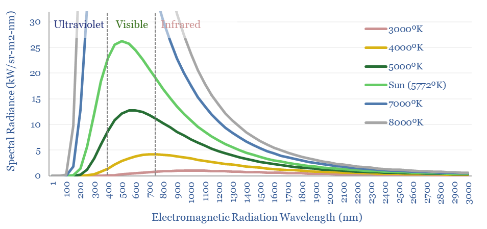
In the chart below, we have run Planck’s equation for radiating bodies at different temperatures from 3,000-8,000ºK, including the sun, whose surface is 5,772ºK. Then we have translated the units into kW per m2 of surface area and per nm of wavelength.
Hence by integration, the ‘area under the curve’ shows the total quantity of electromagnetic radiation per m2. If the surface of the sun were just 10% hotter, then it would emit c50% more electromagnetic radiation and 55% more visible light!
Charts like this also explain why the filament of an incandescent light bulb, super-heated to 2000-3000ºC is only going to release 2-10% of its energy as light. Most of the electromagnetic radiation is in the infra-red range here. And this is the reason for preferring LED lighting as a more efficient alternative. LEDs can reach 60-90% efficiency.
Planck’s Law and Solar Efficiency?
Planck’s Law also matters for the maximum efficiency of a solar module, and can be used to derive the famous Shockley-Queisser limit from first principles, which says that a single-junction solar cell can never be more than c30-33% efficient at harnessing the energy in sunlight.
Semiconductor material has a bandgap, which is the amount of energy needed to promote a single electron from its valence band into its conduction band: a higher energy state, from which electricity can be drawn out of a solar cell. For silicon, the bandgap is 1.1 eV.
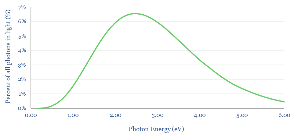
What provides the energy is photons in light. The energy per photon can be calculated according to its wavelength. This involves multiplying Planck’s constant by the Speed of Light, dividing by the wavelength, and then converting from Joules to electronVolts. For a radiating body at 5,772ºK, the statistical distribution of photons and their energies is below.
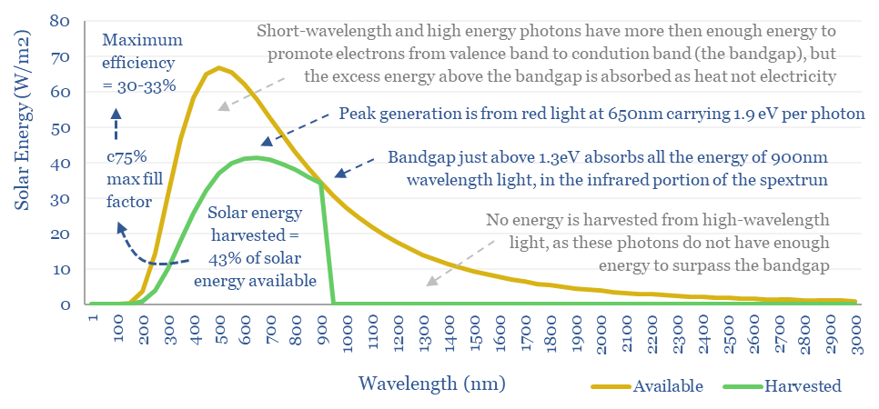
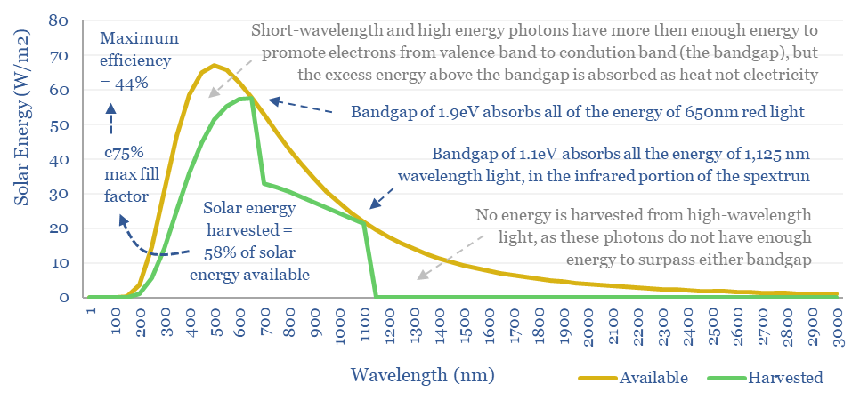
So what bandgap semiconductor is best? If the bandgap is too high (e.g., 4eV), then most of the photons in light will not contain sufficient energy to promote valence band electrons into the conduction band, so they cannot be harnessed. Conversely, if the bandgap is too low (e.g., 0.5eV), then most of the energy in photons will be absorbed as heat not electricity (e.g., a photon with 2.0 eV would transfer 0.5eV into electron promotion, but the remaining 1.5 eV simply heats up the cell).
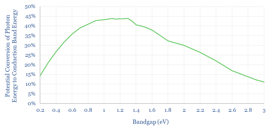
The mathematical answer is that a bandgap just above 1.3 eV maximizes the percent of incoming sunlight energy that can be transferred into promoting electrons within a solar cell from their valence bands to their conduction bands, at 43-44% (chart below).
If we run a sensitivity analysis on the bandgap, the next chart below shows that our 43-44% conversion limit holds for any semiconductors with a bandgap of 1.1-1.35eV, more of a plateau than a sharp peak.
The Shockley-Queisser limit is usually quoted at 30-34%, which is lower than the number above. In addition to the losses due to incomplete capture of photon energy, the maximum fill factor of a solar cell (balancing load, voltage and current) is around 77%, so only 77% x 44% = 34% of the incoming light energy could actually be harnessed as electrical energy. Moreover, in their original 1961 paper, Shockley and Queisser assumed an 87% efficiency limit for impedance matching relative to the 77%, which is why the number they originally quoted was around 30%.
Another issue is that the solar energy arriving at a given point on Earth has been depleted in certain wavelengths, as they are absorbed by the atmosphere. 1,362W/m2 of sunlight reaches the top of the Earth’s atmosphere. While on a clear day, only around 1,000W/m2 makes it to sea level at the equator. We know the atmosphere absorbs specific infrared wavelengths as heat, because this is the entire reason for worrying about the radiative forcing of CO2 or radiative forcing of methane.
Hence for an ultra-precise calculation of maximum solar efficiency, we should not take the Planck curve, but read-out the solar spectrum reaching a particular point on Earth, which will itself vary with weather!!
Multi-junction solar is inevitable?
The biggest limitation on the efficiency of single-junction solar cells is that they only contain a single junction. This follows from the discussion above. But what if we combine two semiconductors, with two bandgaps into a ‘tandem cell’. The top layer has a bandgap of 1.9eV (e.g. perovskite) and the second has a bandgap of 1.1eV (e.g., silicon). The same analysis now shows how the maximum efficiency can reach 44%.
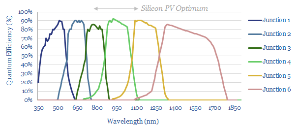
Cells with multiple semiconductors are already being commercialized. For example, we wrote last year about heterojunction solar (HJT) and this year about the push towards perovskite tandems in solar patents from LONGi. It feels like the ultimate goal will be multi-junction cells that capture along the entire solar spectrum (chart below). It will simply take improvements in semiconductor manufacturing.
Elsewhere in the electromagnetic spectrum, this data-file also contains workings into the energy efficiency of microwave energy, transmitting it through space and converting it back to useful electricity via rectennas.
All of the numbers and calculations go back to first principles, in case you are looking to model the Planck Equation, Shockley-Queisser limit, multi-junction solar efficiency, lighting efficiency, or other calculations of electromagnetic radiation energy.
Generac is a US-specialist in residential- and commercial-scale power generation solutions, founded in 1959, headquartered in Wisconsin, with 8,800 employees and $7bn of market cap. What outlook amidst power grid bottlenecks? To answer this question, we have tabulated data on 250 Generac products.
Generac‘s $4bn pa of sales, in 2023, were >50% residential, >35% commercial, 10% other. 80% was domestic within the US, and 20% was international. 12% is attributed to ‘energy technologies’ which includes storage, solar MLPE, EV charging, smart thermostats, electrification, etc. But what about the product mix? How is it exposed to power grid bottlenecks? Or indeed a broader US construction boom?
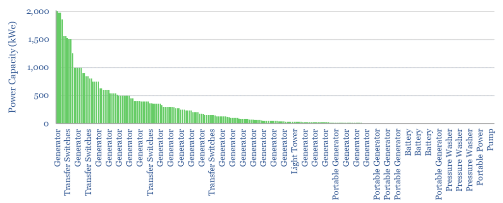
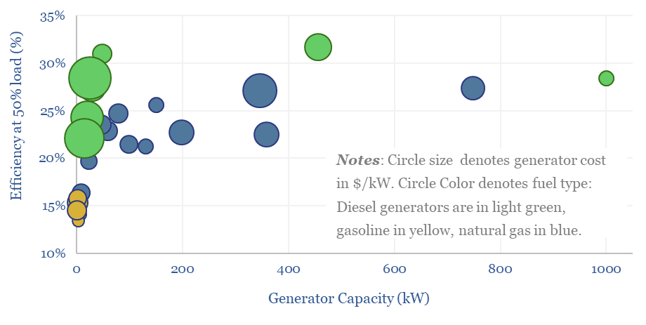
In this data-file, we have tabulated details on 250 Generac Products. 70% are generators, and another c10% are transfer switches to connect generators to loads. Our data show the breakdown of units by size, fuel, prices and other technical parameters.
Residential solutions comprise 55% of Generac’s revenues, as 6% of US homes now have standby generators, but a smaller share of the SKUs. Our data show the average size (in kW), list prices (in $) and costs (in $/kW), but we also think low efficiency in some of these residential generation units is not entirely helpful for decarbonization aspirations.
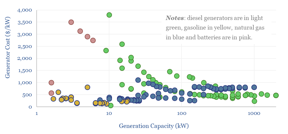
Generac’s larger industrial generators range from 100kW to 2MW in size. Generac’s diesel-fired units cost $500/kW and are c30% efficient, while its larger gas-fired units cost $700/kW and are c25% efficient. These units tend to generate 10-40 kW/m3 of space, and discharge exhaust at 700-800ºC, so they could find application amidst grid bottlenecks?
In our base case model for a diesel genset, we assume a 16-20c/kWh LCOE is needed for a $700/kW installation of a 10MW unit with 42% efficiency buying wholesale diesel. Generac units would appear to have higher costs for reasons in the data-file.
In our base case model for a CCGT, we need a 6.5c/kWh LCOE at an $850/kW installation of a 300MW unit with 55% efficiency buying $4/mcf wholesale natural gas. Again, for the Generac units, we get to a higher LCOE, yes this is the area we think could be most economically justified by growing power grid bottlenecks, especially at industrial facilities that can harness the 700-800ºC waste heat.
Outside of the generation business, remaining SKUs comprise transfer switches to connect generators to loads, pressure washers, light towers for construction, pumps, batteries and mobile heaters, hence there may be heavy exposure to construction and infrastructure projects.
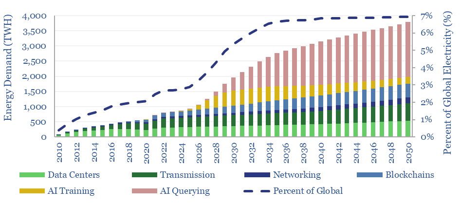
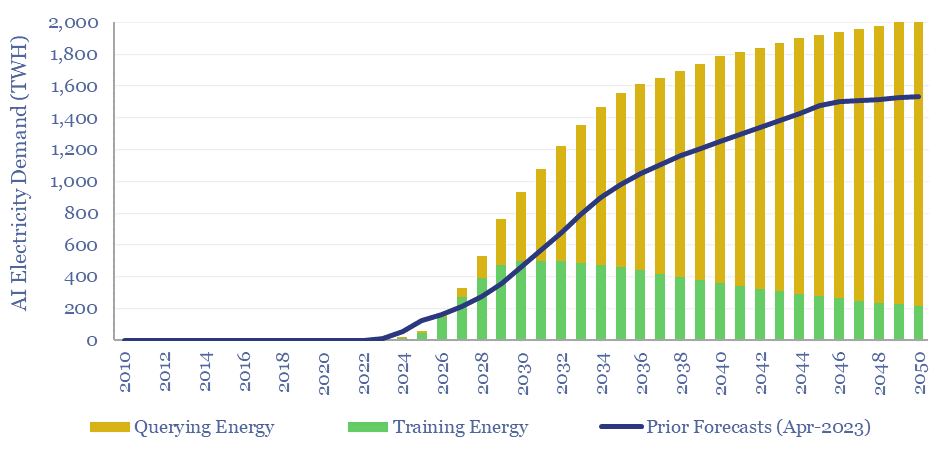
This data-file forecasts the energy consumption of the internet, rising from 800 TWH in 2022 to 2,000 TWH in 2030 and 3,750 TWH by 2050. The main driver is the energy consumption of AI, plus blockchains, rising traffic, and offset by rising efficiency. Input assumptions to the model can be flexed. Underlying data are from technical papers.
Our best estimate is that the internet accounted for 800 TWH of global electricity in 2022, which is 2.5% of all global electricity. Despite this area being a kind of analytical minefield, we have attempted to construct a simple model for the future energy demands of the internet, which decision-makers can flex, based on data and assumptions (chart below).
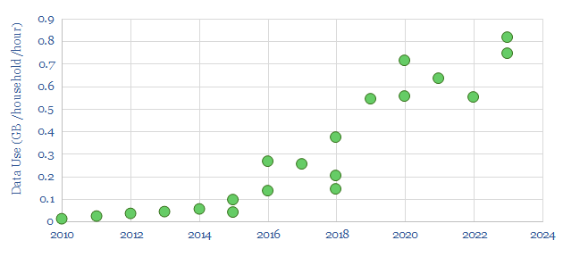
Internet traffic has been rising at a CAGR of 30%, as shown by the data use of developed world households, rising to almost 3 TB per user per year by 2023. The scatter also shows a common theme in this data-file, which is that different estimates from different sources can vary widely.
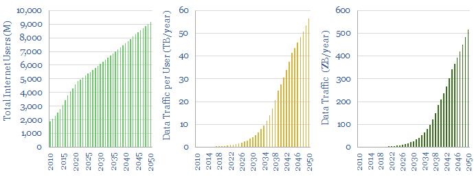
Future internet traffic is likely to continue rising. By 2022 there were 5bn global internet users underpinning 4.7 Zettabytes (ZB) of internet traffic. Users will grow. Traffic per user will likely grow. We have pencilled in some estimates, but uncertainty is high.
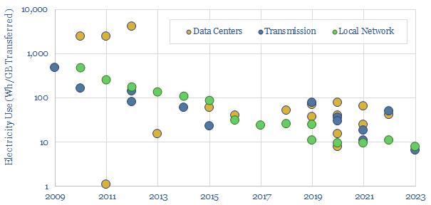
The energy intensity of internet traffic spans across data-centers, transmission networks and local networking equipment. Again, different estimates from different technical papers can vary by an order of magnitude. But a first general rule is that the numbers have declined sharply, sometimes halving every 2-3 years.
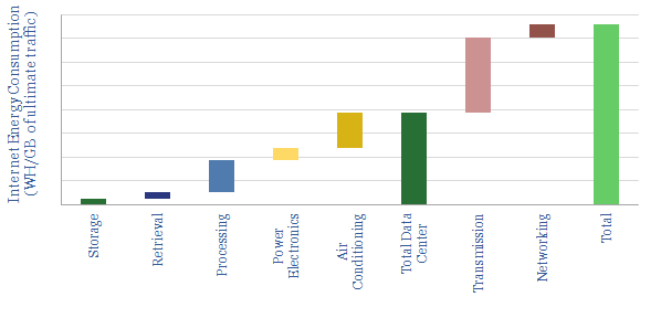
The current energy intensity of the internet is thus estimated at 140 Wh/GB in our base case, broken down in the waterfall chart below, using our findings from technical papers and the spec sheets of underlying products (e.g., offered by companies such as Dell).
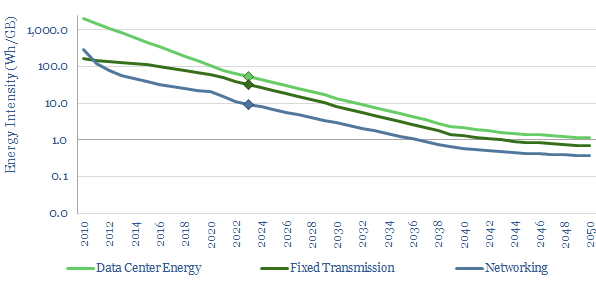
Energy intensity of internet processes will almost certainly decline in the future, as traffic volumes rise. Again, we have pencilled in some estimates to our models, which can be flexed.
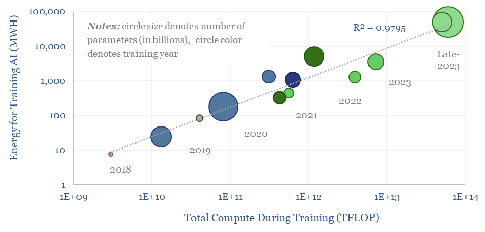
However the energy needed for AI is now rising exponentially. Training Chat GPT-3 in 2020 used 1.3 GWH to absorb 175bn parameters. But training chat GPT-4 in 2023 used 50 GWH to absorb 1.8trn parameters. We find a 98% correlation between AI training energy and the total compute during training.
AI querying energy is also correlated with the complexity of the AI model, and thus will likely continue rising in the future. Average energy use is estimated at 3.6 Wh per query today, which is 4x more than an email (1 Wh) and 10x more than a google search (0.3 Wh).
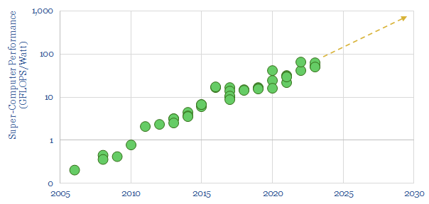
Muting the impacts of larger data-processing volumes, we expect a 40x increase in future computer performance in GFLOPS per Watt (chart below). This yields 900 TWH of AI demand around 2030, revised up from 500 TWH in April-2023 (chart above).
Please download the model to stress-test your own estimates for the energy intensity of the internet. It is not impossible for total electricity demand to ‘go sideways’ (i.e., it does not increase). It is also possible for the electricity demand of the internet to exceed our estimates by a factor of 2-3x if the pace of productivity improvements slows down.
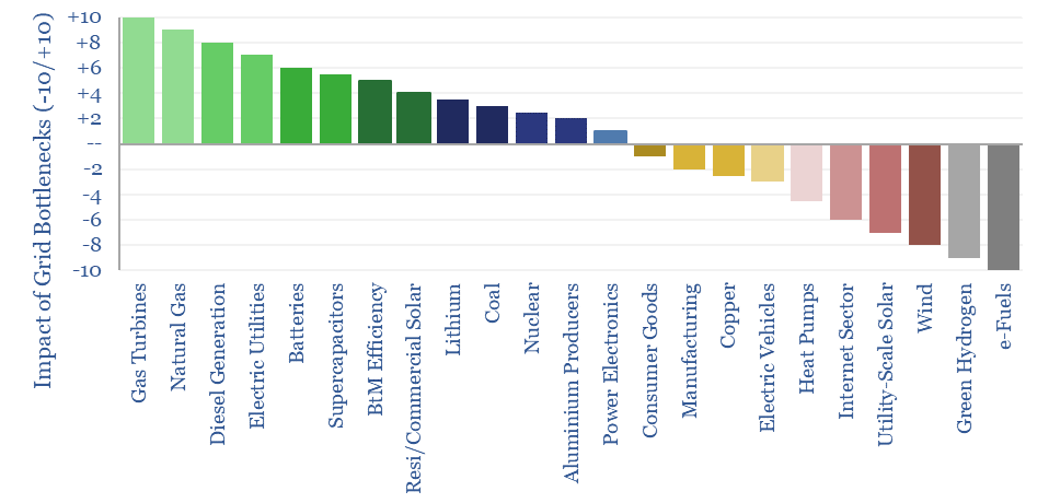
What if the world is entering an era of persistent power grid bottlenecks, with long delays to interconnect new loads? Everything changes. Hence this 16-page report looks across the energy and industrial landscape, to rank the implications across different sectors and companies.
Cookies?
This website uses necessary cookies. Our cookies are simply to improve your experience. We do not undertake any advertising or targeting via our cookies. By clicking 'accept' or continuing to use the website, you consent to our use of cookies.AcceptRead More
Privacy & Cookies Policy
Privacy Overview
This website uses cookies to improve your experience while you navigate through the website. Out of these, the cookies that are categorized as necessary are stored on your browser as they are essential for the working of basic functionalities of the website. We also use third-party cookies that help us analyze and understand how you use this website. These cookies will be stored in your browser only with your consent. You also have the option to opt-out of these cookies. But opting out of some of these cookies may affect your browsing experience.
Necessary cookies are absolutely essential for the website to function properly. This category only includes cookies that ensures basic functionalities and security features of the website. These cookies do not store any personal information.
Any cookies that may not be particularly necessary for the website to function and is used specifically to collect user personal data via analytics, ads, other embedded contents are termed as non-necessary cookies. It is mandatory to procure user consent prior to running these cookies on your website.