Downloads Insights- Thunder Said Energy

DAC companies: direct air capture screen?

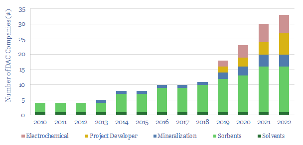
Leading direct air capture companies (DAC companies) are assessed in this data-file, aggregating company disclosures, project disclosures and other data from patents and technical papers. The landscape is evolving particularly rapidly, trebling in the past half-decade, especially towards novel DAC solutions.

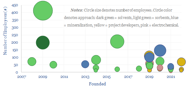
Most of the DAC companies in this data-file are private, with an average of c65 employees, and focuses ranging across L-DAC, S-DAC, CO2 mineralizations, project development and novel electrochemical approaches. The data-file covers each company, its approach, headquarters, employee count, capital raising and recent news that stood out to us.

Half a decade ago, the DAC company landscape was dominated by well-known leaders, such as Carbon Engineering, Climeworks and Global Thermostat (all founded in 2009-2010).

However in the past half-decade, the size of the space has trebled, with a clear focus upon next-generation DAC designs (or as we call it, ‘DAC to the future‘) which could confer materially lower energy intensities and financial costs, using advanced sorbents, passive DAC, mineralization and electrochemical systems. Many are at the pilot stage.

Large projects are compiled in the projects tab, ranging from Climeworks’ 4kTpa Orca demonstration plant that started up in 2021 using geothermal energy in Iceland; through to the first 1MTpa-scale projects being progressed by 1PointFive, the consortium between Occidental and Carbon Engineering. The largest proposed project we have seen is 5MTpa.

Modularity is also a growing topic amongst emerging DAC companies, which may not build MTpa-scale plants but tens of thousands of 10-1,000 Tpa modules, which will be cheaper to manufacture and can integrate with other facilities.

Electrochemical DAC excites us most and we will undertake TSE patent reviews into some of these companies in due course.

Battery cathode active materials and manufacturing?

Lithium ion batteries famously have cathodes containing lithium, nickel, manganese, cobalt, aluminium and/or iron phosphate. But how are these cathode active materials manufactured? This data-file gathers specific details from technical papers and patents by leading companies such as BASF, LG, CATL, Panasonic, Solvay and Arkema.

New energies are entering an age of materials, where an increasing share of costs are accruing to materials companies, while more advanced materials hold the key to continued efficiency gains and cost deflation (per our research note below).

There is a mild temptation to gloss over the complexity of manufacturing battery cathodes, as though you ‘just get some metals and wop them in’. The reality is a complex, ten step process, which also explains some of the challenges ahead for battery recycling.

New energies: the age of materials?

Cathode manufacturing: ten-stage process?

(1) Lithium is sourced as lithium hydroxide or lithium carbonate in the first stage of manufacturing a lithium ion battery cathode.

(2) Lithium inputs are then combined with transition metals and other additives. The transition metals may include nickel, manganese, cobalt, or iron phosphate precursors. Different cathode chemistries and their resultant properties are covered in this data-file.

Lithium ion batteries: breakdown of materials?

(3) Precursor cathode active materials are then typically heated in an oxygen enriched atmosphere for c12-hours at c700ºC. The aim is to calcine away impurities and form coherent metal oxide crystals. Energy use is likely 60-100 kWh/kWh of batteries, per our data-file here. Variations are discussed in the data-file.

(4) Next may follow various stages of sieving, crushing-grinding, acid-treating, dosing with additives, washing and drying, to modify the outer surface of the cathode active materials. The details also vary quite widely between patents in the data-file.

(5) Next the Cathode Active Materials, which are typically 92% of the weight of a finished battery cathode, are mixed with a conductive carbon additive, most often carbon black, but also potentially graphite or carbon nanotubes, which will typically form 5% of the cathode.

(6) A fluorinated polymer binder, most often PVDF is also sourced. This is an inert plastic that physically holds all of the other the active materials together and will typically form 4% of the cathode. PVDF is also used to bind graphite at the anode.

Fluorinated polymers: flying under the radar?

(7) All of these Cathode Active Materials are then dissolved in a solvent, typically N-Methyl-2-Pyrrolidone (NMP), to form a mixed slurry of c60% solids, c40% NMP.

(8) The slurry is deposited onto a 10-20μm thick aluminium current collector (for contrast, the anode side of the cell tends to use a thinner, copper current collector).

(9) The NMP is then evaporated and recovered by heating for 12-hours at 110ºC. Note this is below the 200ºC boiling point of NMP, because PVDF binder is only rated to 120ºC. Hence the process may require a mild vacuum and long heating times so evaporation can occur via Boltzmann statistics (chart below). Energy use is likely 20-40 kWh/kWh, again per our data-file here.

The resultant battery cathode will typically have a thickness of 70μm, containing 15 mg/cm2 of active material.

(10) Half-cell manufacturing. To prevent oxidation of the cathode, some processes then immediately manufacture half-cells under an inert atmosphere (e.g., nitrogen, argon). Electrolyte is added to the half-cell, most often by dissolving the ionic salt LiPF6 at 1M concentration in a mixed solvent of ethylene carbonate, ethyl methylene carbonate, di-ethylene carbonate, propylene carbonate, et al. Then a polymer separator is added. The average finished battery cell is 3.5mm thick.

Cathode manufacturing: leading companies?

Two companies stood out as having filed the most patents into battery cathode active materials and manufacturing, often departing quite materially from the simplified description above, suggesting a proprietary process? Details in the data-file.

Materials companies also stood out in the patents and technical papers, as the same companies were often listed as supplying high-grade materials. For example, PVDFs from Solvay, and carbon black from Imerys, although we also wonder about using Huntsman’s new MIRALON product here. Details of metals suppliers, NMP suppliers, separator suppliers and niche equipment suppliers are in the data-file.

Solvay: lithium ion battery binders and additives?

Solvay is a chemicals company with growing exposure to battery materials, especially the PVDF binders that hold together active materials in the electrodes. But also increasingly in electrolyte solvents, salts and additives. Interestingly, our patent review finds optimizations of this overall system can improve the longevity and energy density of batteries, which may also lead to consolidation across the battery supply chain?

Solvay is a chemicals company, listed in Brussels and Paris, with history dating back to 1863, 22,000 employees, €13.4bn of revenues in 2022, 24% EBITDA margin and €11bn of market cap at the time of writing in September-2023.

Its Materials segment produces specialty polymers and composites for light-weighting vehicles and aerospace parts; its Chemicals business produces soda-ash, peroxides, silica, et al; and its Solutions business produces specialty chemicals, aromas, coatings, Rare Earths, mining solutions and battery recycling.

For the energy transition, Solvay is a leading producer of battery binders, which are fluorinated polymers, mainly PVDF, that physically bind the metal particles together in a battery cathode and the graphite particles together in a battery anode. Solvay has the broadest PVDF offering in the battery materials space, spanning across both suspension- and emulsion technologies. And it is investing to expand capacity in France, the US and China. We found some interesting battery binder innovations in the patents.

However what surprised us most about reviewing Solvay’s patents was that there was 2x more focus on developing battery electrolytes and additives than on improving binders. Typically, the electrolyte of a lithium ion battery consists of LiPF6, an ionic salt, which is dissolved in ethylene carbonate, dimethyl carbonate or vinylene carbonate. However, this also places a limit on the battery energy density (and by extension, materials intensity), as most of these solvents start decomposing at 4.2-4.4V. For more details, please see our deep-dive report into battery degradation.

The patents strongly imply that electrodes, binders, electrolyte solvents, salts and additives form an ‘overall system’ where all of the components interact. Hence as the battery industry focuses upon lower degradation and higher voltage (more energy dense) battery chemistries, we wonder if this will drive consolidation across the supply chain, where battery manufacturers will want to buy all of these mutually interactive materials as part of an overall offering from a single integrated supplier rather than purchasing them separately?

Overall Solvay’s battery patent library is complex, with literally hundreds of different electrolyte salts, solvents and additives and blended together in cocktails. Over 90% of the patents provided specific details of specific compositions, aimed at improving cell longevity, or voltage, or efficiency (charts below).

Back in the world of battery binders, there is also a side focus on developing lithium metal batteries, or solid state batteries. Note that a typical lithium ion battery uses fluorinated polymer binders in its electrodes, but a solid state battery would use fluorinated polymer binders in its electrolyte too.

Please download the data-file for further conclusions from our Solvay battery technology review, and conclusions on whether the company has a moat around its patents.

Jevons Paradox: what evidence for energy savings?

Using a commodity more efficiently can cause its demand to rise not fall, as greater efficiency opens up unforeseen possibilities. This is Jevons’ Paradox. Our 16-page report finds it is more prevalent than we expected. Efficiency gains underpin 25% of our roadmap to net zero. To be effective, commodity prices must also rise and remain high, otherwise rebound effects will raise demand.

Energy Recovery Inc: pressure exchanger technology?

A pressure exchanger transfers energy from a high-pressure fluid stream to a low-pressure fluid stream, and can save up to 60% input energy. Energy Recovery Inc is a leading provider of pressure exchangers, especially for the desalination industry, and increasingly for refrigeration, air conditioners, heat pump and industrial applications. Our technology review finds a strong patent library and moat around Energy Recovery’s pressure exchange technology.

Energy Recovery Inc was founded in 1992, it is headquartered in California, listed on NASDAQ, with 250 employees and $1.3bn of market cap at the time of writing. Financial performance in 2022 yielded $126M revenues, 70% gross margin, 20% operating margin.

The PX Pressure Exchanger is Energy Recovery Inc’s core product. It transfers pressure energy from a high pressure fluid stream to a low pressure fluid stream at 98% efficiency, yielding up to 60% energy savings in specific contexts. The company aims to grow revenues as much as 5x in the next half-decade due to increasing need for global energy efficiency.

Pascal’s Law states that bringing a high pressure and low pressure fluid into contact will result in their pressures equalizing with minimal mixing. This principle is used in pressure exchangers. As a rotor rotates, it brings a low pressure fluid A into contact with a high pressure fluid B, equilibrating their pressure, then discharging fluid A at higher pressure.

For example in a desalination plant, incoming seawater at 1-3 bar of pressure is pressurized up to 40-80 bar using pumps, pushing it across a membrane that is porous to water but not to dissolved salts. Energy remains in this 40-80 bar concentrate stream. It is better to recover this energy than blast it back into the Ocean! Thus pressure exchange can lower the energy requirements of desalination by as much as 60%.

Energy Recovery Inc’s patents note that rotary pressure exchangers were first invented in the 1960s, progressed in the 1990s, but prior to its own designs, the company argues that no one had designed efficient and reliable systems, which could run without an external motor to rotate them, achieved by optimizing the shape of the flow channels.

Our technology review found 65 patent families from Energy Recovery Inc. Overall, we think the patent library is high-quality and the company will retain a moat and leadership in the pressure exchange market, based on its patents and historical experience. Although some early patents are coming up to expiry. Details are in the data-file.

Desalination has been Energy Recovery’s core market historically. However new markets are emerging, from cryogenic cycles through to applications focused on shale (although the latter requires avoiding the corrosive impacts of sand and debris in fluid streams).

Refrigeration, air conditioning and heat pumps are seen as a growing source of demand. One patent notes that regulation is increasingly phasing out HFCs that can have 13,000x higher GWPs than CO2, and these systems use CO2 as the refrigerant instead. However CO2 based refrigeration cycles have maximum pressures of 1,500 psi or greater, compared to HFC/CFC systems at 200-300psi. This makes the energy savings from pressure exchange increasingly important, siphoning away a portion of the evaporated refrigerant and re-pressurizing it using high-pressure refrigerant downstream of the heat rejection stage, before the expansion valve stage.

Average home sizes: living space per person?

Average home sizes matter for overall residential energy demand, heating and cooling demand. Hence the purpose of this data-file is to aggregate average home sizes by country, then translate the data into living space per capita. A good rule of thumb is that each $1k pp pa of GDP translates one-for-one into 1m2 pp pa of useful living space. The trend towards ever larger homes challenges the notion of peak energy demand?

On a global average basis, the average home is 70m2 in size and shared between 3.5 inhabitants, which equates to an average of 20m2 of living space per capita.

There is a direct linear relationship between income per capita and living space per capita. A good rule of thumb is that each $1k of GDP per capita equates to 1m2 per capita of living space.

In wealthy countries, the average home is 130-200m2 in size, shared between 2-2.5 people, for an average of 60-80m2 of living space per person, which is 3x the global average. This is large, but still not that large. A mansion is 800m2 and above. The largest houses in the US are catalogued here. And the largest house in the world, belonging to the Sultan of Brunei, is 200,000m2.

In the least wealthy countries, the average home is 20-40m2 in size, shared between 3-5 people, and thus living space per capita is 5-10m2, 50-75% below the global average. This is staggeringly low. For example, a recent press article highlighted that the average living space per capita in a dwelling in India is “less than the recommended size of a prison cell”.

Average home sizes have been increasing in substantively every country we surveyed. For example, the average new single-family home being built in the United States in 2022 is 223 m2, up 45% since 1980, up 2.5x since 1900. Household sizes have fallen from 4.8 people in 1900 to 2.5 people in 2022. Hence overall, total living space per American in these newly built homes has risen by 60% since 1980 and 5x since 1900 (charts below).

In my adopted homeland of Estonia, I have also seen my fair share of boxy 30-40m2 concrete monstrosities, dating back to the fifty year period of Soviet occupation. No one really wants to live in them. The average size of a new dwelling constructed in 2023 has jumped to 83 square meters.

Urbanization patterns are another driver of average home sizes. A typical urban apartment is about half the size of a typical ‘house’. However another demographic trend is that wealthier urbanites tend to move out of apartments and ‘out into the suburbs’ which also adds energy demand in the form of commuting.

Overall we think that rising home sizes are another example of a rebound effect severely challenging the idea of ‘peak energy demand’. Improved living standards, building materials, efficiency, insulation, heating and cooling, will almost invariably result in people choosing to live in larger houses, which in turn consume more energy.

The data in this file are the best aggregation we could find from technical papers, national records, internet searches, and data-based triangulation. As far as we are aware, there is no aggregated source of home sizes released by global statistical agencies.

Countries covered in the data-file include Argentina, Australia, Bangladesh, Bolivia, Brazil, Canada, China, Colombia, Congo, Denmark, Egypt, Estonia, Finland, France, Germany, Greece, Hong Kong, India, Indonesia, Italy, Japan, Korea, Mexico, Netherlands, New Zealand, Nigeria, Norway, Poland, Portugal, Romania, Russia, South Africa, Spain, Sweden, the United Kingdom, the United States and Vietnam.

Shale oil: fractured forecasts?

This 17-page note makes the largest changes to our shale forecasts in five years, on both quantitative and qualitative signs that productivity growth is slowing. Productivity peaks after 2025, precisely as energy markets hit steep undersupply. We still see +1Mbpd/year of liquids potential through 2030, but it is back loaded, and requires persistently higher oil prices?

Residential energy consumption over time?

US residential energy consumption runs at 3,000 MWH per annum, equivalent to one quarter of total US energy consumption. Total demand has run sideways since 1980 as rebound effects and new demand sources have offset underlying efficiency savings?

This data-file compiles a time-series of US residential energy consumption over time, based on periodic surveys conducted every 3-7 years by the US EIA.

US residential energy consumption is around 3,000 MWH per annum, equivalent to 9 MWH per person per year, up on 1980 in absolute terms, but down 30% since 1980 in per capita terms.

US residential electricity consumption has increased from 3 MWH pp pa in 1982 to 4 MWH pp pa in 2022.

Efficiency gains are visible in categories such as refrigeration, where electricity consumption has fallen from 0.7 MWH pp pa in 1982 to 0.3 MWH pp pa in 2022.

On the other hand, new categories of demand, such as air conditioning and other appliances, have more than offset the efficiency improvements in individual devices such as refrigerators.

Heating demand for houses has halved from 120 kWh per m2 of living space per annum in 1980 to 60 kWh per m2 of living space per annum in 2022, due to improving insulation.

However, rebound effects are also visible in this category, as new single-family homes have become 60% larger over the same timeframe.

Finally, the data-file contrasts residential electricity consumption in the US versus other geographies. Statistically, a hot tub in the Alps consumes more electricity per annum than an African village of 40 people.

Data are aggregated in the Excel file as a useful reference running back to 1980. For more, please see our research into rebound effects and Jevons Paradox and our overall US energy supply demand model.

Fans and blowers: costs and energy consumption?

Fans and blowers comprise a $7bn pa market, moving low-pressure gases through industrial and commercial facilities. Typical costs might run at $0.025/ton of air flow to earn a return on $200/kW equipment costs and 0.3kWh/ton of energy consumption. 3,000 tons of air flow may be required per ton of CO2 in a direct air capture (DAC) plant.

Fans and blowers comprise a $7bn pa global market, moving large volumes of air for industrial and commercial purposes, at pressure closer to atmospheric pressure (up to 1.11x pressurization for a fan, up to 1.2x pressurization for a blower).

A good rule of thumb is that moving 1 ton of air through an industrial facility ‘costs’ 2.5 cents, using 0.3 kWh/ton of electricity and in order to re-coup a return on a $200/kW investment (as aggregated from equipment providers, chart below).

However, these numbers can all vary, rising considerably when there is more resistance in the system, and fans/blowers must work to overcome larger total pressure drops. The simple energy economics are that power consumption (in Watts, aka Joules per second) is a product of air flow (in m3/second) x the total pressure increase imparted to the air (in Pa, aka J/m3). In turn, the dynamic pressure rise is a square function of flow velocity.

The economic costs and energy costs of blowers and fans might sound small, but note that a direct air capture (DAC) plant will need to move something like 3,000 tons of air per ton of CO2 that is captured, which could cost $75/ton and 300-900kWh/ton of electricity just circulating air through the plant.

As a comparison, compressors typically step up gas pressures from 2-100x depending on the application, with costs around $850/kW in a $140bn pa global market today.

Underlying data into the capex, energy consumption and volumetric flow rates are tabulated in the tabs overleaf, simply aggregating public disclosures across companies supplying fans and blowers.

Gas fractionation: NGL economics?

$Gas fractionation$

Gas fractionation separates out methane from NGLs such as ethane, propane and butane. A full separation uses up almost 1% of the input gas energy and 4% of the NGL energy. The costs of gas fractionation require a gas processing spread of $0.7/mcf for a 10% IRR off $2/mcf input gas, or in turn, an average NGL sales price of $350/ton. Costs of gas fractionation vary and can be stress tested in this model.

Wellhead gas is mainly composed of methane, it also contains propane, butane, C5s and C6+ fractions, which are entrained in the gas. These condensates or natural gas liquids (NGLs) can be removed by first dehydrating the gas, then, cryogenically cooling it, to ‘drop out’ all of the NGL fractions in a demethanizer (chart below). (For more details, we have written an overview of cryogenics)

The NGLs may then be heat exchanged with steam or warm oils, to warm them back up, and fractionate out the components: with ethane evaporating first in the de-ethanizer (boiling point is -89 °C), next propane in the depropanizer (boiling point is -42ºC) and butane next in a debutanizer (-1ºC). There may be separate stages to separate n-butanes from i-butanes.

The process can vary. Some facilities only drop out mixed NGLs, which are then shipped onwards. Others will cool the gas to separate out C3+, but will leave the ethane entrained, due to limited ethane uses outside of ethane crackers. You can flex these options in the data-file. But our base case captures a full separation of all NGL fractions.

Energy costs of full natural gas fractionation will come to 113kWh/ton of input gas (using up 1% of its energy content) and 600kWh/ton of NGLs (using up 4% of its energy content).

Capex costs of full natural gas fractionation can be estimated with the simple rule of thumb of around $1M/mmcfd of demethanizer capacity plus $5M/kbpd of NGL fractionation capacity. This is based on past projects, tabulated in the data-file.

The costs of a natural gas fractionation plant require a fractionation spread of $0.7/mcf of input gas processed, in order to separate all the NGL fractions and earn a 10% IRR. In other words, if the input gas price is $2/mcf, then the fractionation plant needs to charge a blended average of $2.7/mcfe on sales gas and the various NGL products.

What NGL prices are needed for a 10% IRR? At $2/mcf, our model requires a blended price around $350/ton, across ethane, propane, butanes, and higher fractions. Recent pricing is below, based on data from the EIA. Each $1/mcf on the gas price requires a further c$80/ton onto the required average NGL price.

NGL fractionation is increasingly important to provide feedstocks for advanced polymers used in new energies and energy efficiency technologies. But we also see a growing role for low-carbon natural gas in the energy transition. And fractionation is usually done before natural gas is liquefied into LNG.

Leading companies operating natural gas fractionation plants are constellated around the upstream and midstream industries, while companies such as Technip, Linde, Lummus and other industrial gas companies and oil service companies supply equipment and technology for NGL fractionation plants.

Cathode manufacturing: ten-stage process?

Cathode manufacturing: leading companies?

Cookies?