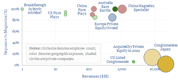
The global magnet industry is fragmented across hundreds of suppliers, including 800 in Asia-Pacific. The total market is worth $20bn pa. The purpose of this data-file is to highlight a dozen leading magnets and permanent magnets companies, including Rare Earth magnets (e.g., NdFeB), ferrites and other magnetic components.
More mundanely, permanent magnets are also sold into ordinary household appliances like tumble dryers; and electronics such as iDevices and audio equipment. Indeed, the largest specialist magnets companies in our screen sell products to over 2,000 active customers, ranging from <1mm micro-magnets to 200mm monsters, with energy products from 1-60 MGOe.
High competition is borne out by middling margins, which tend to average c20% at the EBITDA level, c10% at the EBIT level and single digits at the net level. Although further upstream, Rare Earth miners have recently generated EBITDA margins closer to 50%, and expanding. There may also be higher margins for specialized and premium companies.
Private permanent magnets companies. An interesting trend in the screen is rising private equity activity. For example, a consortium led by Bain Capital acquired Hitachi Metals in 2022, and re-spun the company as Proterial in early 2023.
Listed pure-play permanent magnets companies in the screen include two Chinese Rare Earths magnet-makers, and a $5bn Australian Rare Earths miner.
Diversified companies are also noted in the screen, with Rare Earths, magnetic materials or magnet components as part of the broader commercial portfolios, including a leading Japanese large-cap.
An overview of all of these companies, as well as an overview of energy and magnetism, is also given for TSE written subscription clients in our recent research note here. Useful industry data-points behind the note, such as different magnet types and their typical properties and magnet costs ($/kg), are also compiled in the data-file.
The DRI+EAF pathway already underpins 6% of global steel output, with 50% lower CO2 than blast furnaces. But could IRA incentives encourage another boom here? Blue hydrogen can reduce CO2 intensity to 75% below blast furnaces, and unlock 20% IRRs at $550-600/ton steel? This 13-page report explores the opportunity, and who benefits.
Electra is developing an electrochemical refining process, to convert iron ore into high purity iron, and ultimately into steel, using only renewable electricity. It has raised c$100M, gained high-profile backers, and is working towards a test plant. This 9-page note is an Electrasteel technology review, based on an exceptionally detailed patent, finding clear innovations, but also some remaining risks and cost question marks.
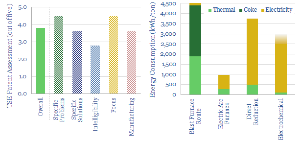
Global steel production has risen by 10x since 1950, to 2GTpa by 2022, and demand is still rising at 2.5% per year since 2012. 70% of steel is made in blast furnaces and basic oxygen furnaces, in a pathway that emits over 2 tons of CO2 per ton of finished steel (model here). Hence the steel industry comprises 8% of global CO2 emissions.
Blue steel can be made by increasing the portion of blue hydrogen blending in directly reduced iron and electric arc furnaces, in a process that is already technically mature, comprises 6% of global steel production, and can yield 50-75% decarbonization of steel with minimal additional costs, and with a possible IRA-triggered boom on the way (note here).
Green steel can also be made via a similar pathway to DRI+EAFs and blending in green hydrogen as the reducing agent. In the past, we worried that this pathway would be overly expensive, and cause some inflationary circular reference errors in new energies value chains (note here).
Electra’s iron ore reduction process is an alternative method for steel production using only renewable electricity. It uses a proton exchange membrane electrolyser to generate protons from water, uses the protons to acidically dissolve Fe3+ ions from iron ores, electrochemically reduces Fe3+ to Fe2+, then purifies the Fe2+ ions, filters them to a separate electrowinning cell, and plates out pure Fe metal. This is patent protected.
This 9-page report is our Electrasteel technology review, based on a particularly detailed patent that we have assessed on our usual framework (pages 1-2). It covers in detail how we think Electrasteel’s technology works (pages 3-5), where we think the patents point to a breakthrough (page 6), possible energy intensity (page 7), renewable steel costs (page 8) and remaining technical challenges that need to be de-risked (page 9).
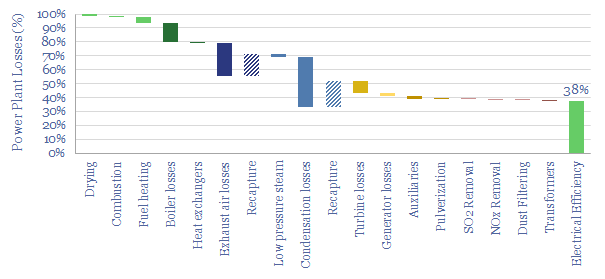
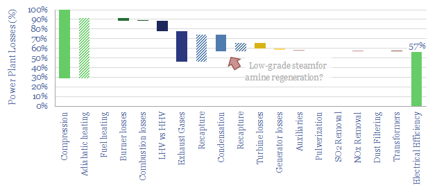
This data-file is a simple loss attribution for a thermal power plant. For example, a typical coal-fired power plant might achieve a primary efficiency of 38%, converting thermal energy in coal into electrical energy. Our loss attribution covers the other 62% using simple physics and industry average data-points.
In our power plant loss attribution, the largest losses are modeled to occur in the steam condensation stage of the Rankine Cycle (17% of losses), the boiler (14%), turbine losses (9%), heat lost in exhaust air (8%), fuel heating (4%), generator losses (2%), plant auxiliaries (2%), and other smaller losses, including incomplete combustion, fuel drying, fuel milling, flue gas desulfurization, NOx removal via selective catalytic reduction, dust removal via electrostatic precipitators and electrical losses such as transformers.
A range of typical efficiency factors are summarized from technical papers. But a reasonable base case might include 86% boiler efficiency, 90% turbine efficiency, 97% generator efficiency and 8.5% auxiliary losses (note the denominators differ case-by-case, as shown in the data-file).
Thermal power plant efficiency can vary from 20% to 50%. You can stress test different variables in rows 30-46, in order to test rules of thumb over the thermal efficiency of power plants.
Heat recovery. A massive 60% of a thermal power plant’s gross thermal energy ends up being imparted into hot exhaust gases from the boiler, and low pressure steam exiting a cascade of turbines. This is waste heat. The recapture of waste heat is the largest determinant of the efficiency of a thermal power plant. Our base case model assumes that 50% of the low-pressure steam heat and two-thirds of the exhaust gas waste heat is recaptured via heat-exchangers (e.g. warming up input air, fuel and cold water entering the boilers). Without this heat recovery, the thermal efficiency of our coal-fired power plant would be a pathetic 3%. And indeed, sub-10% efficiency factors were common from the dawn of the industrial revolution through to the start of the 20th century (data here). A 10pp increase in heat recovery raises our efficiency factor by 3% from 38% to 41%. However, in practice, this will also require higher capex.
Unit efficiency. Efficiency can be uplifted by around 4%, to 42%, by replacing average boilers, turbines, generators and auxiliary loads with best-in-class boiler efficiency, turbine efficiency, generator efficiency and auxiliary loads. However, in practice, this will also require higher capex.
Hotter cycles. Our base case model is a supercritical cycle around 566◦C, however, varying the maximum temperature of the cycle by +/- 100◦C changes the cycle efficiency by +/- 1%. The reason is that less working fluid is needed for a hotter cycle, which lowers the losses involved in evaporating and then re-condensing water; there is simply less water.
Hotter ambient temperatures. Our base case model assumes an ambient temperature of 20◦C. However, when ambient temperatures are 40◦C, efficiency falls by 0.3%, because it becomes harder to extract as much heat from the working fluid as it expands across the turbines and in the process cools towards ambient temperatures.
Higher-grade fuel. Coal grades vary. But generally, coal needs to be heated to above 400◦C to ignite, and above 500◦C to auto-ignite (data here). Replacing high-grade bituminous coal (6,500 kWh/ton) with low-grade lignite (3,500 kWh/ton) will lower efficiency by around 3%, because of the additional fuel-heating that is required.
Wetter fuel. Similar rules apply to fuels with a higher moisture content, as this moisture needs to be evaporated. Our base case coal has 10% moisture content, whereas a coal with 20% moisture content will lower efficiency by 0.3%.
Exhaust gas regulations. We think that 1.3% of the plant’s electricity will be lost in meeting developed world flue gas regulations, which require SO2 removal via flue gas desulfurization, NOx removal via selective catalytic reduction and dust removal via electrostatic precipitators. However, some thermal coal plants do not face exhaust gas regulations. Others face even more stringent regulations.
Biomass fired power. We have also developed a biomass-fired variant of the model, reflecting the lower thermal energy of wood versus coal, the higher moisture content and a lower combustion temperature. The base case thermal efficiency of a wood-fired power plant is 34%.
Gas turbines. We have also developed a gas-turbine variant of the model, reflecting the energy economics of the Brayton cycle from first principles, as a function of compression ratios and temperatures across the cycle. The base case thermal efficiency is 40% for a simple cycle gas turbine, rising to 57% efficiency for a combined cycle gas turbine (chart below). Here is hoping that this simple model of gas turbine efficiency is useful. Intriguingly, we think that the energy penalties for gas-fired CCS are only around 10-20%, versus 40% for CCS at power plants combusting solid fuels. For simple cycle gas turbines, the amine reboiler duty can often be met entirely via waste heat.
All of the variables above can be stress-tested in the data-file, which serves as a simple power plant loss attribution. The discussion above highlights that thermal power plants can have efficiencies anywhere from 20-60% depending on their configuration.
Electrostatic precipitator costs can add 0.5 c/kWh onto coal or biomass-fired electricity prices, in order to remove over 99% of the dusts and particulates from exhaust gases. Electrostatic precipitators cost $50/kWe of up-front capex to install. Energy penalties average 0.2%. These systems are also important upstream of CCS plants.
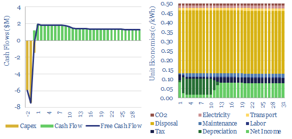
This data-file captures electrostatic precipitator costs, in order to remove particulate dusts from exhaust gases, especially in coal-fired power plant applications. As usual, we model what power plant increment is required to earn a 10% IRR on the up-front capex, opex and other costs of an air pollution control installation.
What is an electrostatic precipitator? ESPs flow exhaust gases through a honeycomb of tubes. Each tube contains a high-voltage wire, creating an electrical corona, imparting a charge to passing dust particles. The charged dust particles will then be attracted towards collecting plates, from which the dust can later be collected via rapping the plates (dry precipitators) or spraying the plates (wet precipitators).
Our base case cost estimate is that an electrostatic precipitator can add 0.5 c/kWh to the costs of a coal-fired power plant, to earn a 10% IRR on an ESP costing $50/kW, and incurring a 0.2% total energy penalty.
However, two-thirds of our cost build-up reflects subsequent disposal of captured dusts and particulates, especially where these dusts contain heavy metals. Not all facilities will incur these costs. Landfill costs vary by region. Trucking costs depend on distance. And different coals have different contaminants. Thus disposal costs can be flexed in the model.
The Electrostatic Precipitator market is approaching c$10bn per annum. It is increasingly important in the energy transition, as exhaust gases require large amounts of clean-up upstream of post-combustion CCS plants, to prevent releases of amines or their breakdown products, which can be problematic for air permitting and air quality. Also important for CCS stability are flue gas desulfurization (remove SO2) and selective catalytic reduction (remove NOXs).
Leading companies in electrostatic precipitators are briefly discussed on the ‘notes’ tab. The market includes industrial giants (Mitsubishi, GE, Siemens Energy, Alstom) through to more specialized companies that have historically installed over 5,000 air pollution control systems worldwide (Babcock, FLSmidth, Ducon, Wood Group).
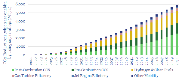
Super-alloys have exceptionally high strength and temperature resistance. They help to enable 6GTpa of decarbonization, across efficient gas turbines, jet engines (whether fueled by oil, hydrogen or e-fuels), vehicle parts, CCS, and geopolitical resiliency. Hence this 15-page report explores nickel-niobium super-alloys, energy transition upside, and leading companies.
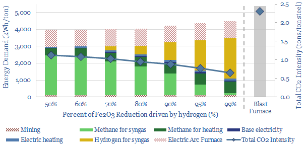
Direct reduced iron (DRI)is produced by reacting iron ore with H2-rich syngas, fueled by natural gas, in over 150 facilities worldwide. Direct reduced iron costs $300/ton, consuming 3,000kWh/ton of energy and 0.6 tons/ton of CO2. The process can be decarbonized via low-carbon hydrogen, as the world strives towards decarbonized steel.
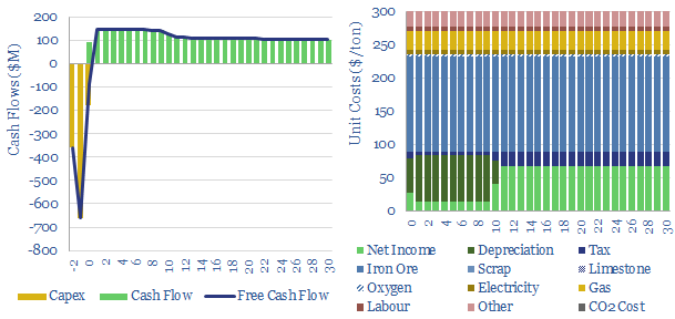
This data-file is an economic model of direct reduced iron (DRI) costs, including a breakdown of capex, opex, natural gas, electricity, iron ore, other materials, labor and taxes.
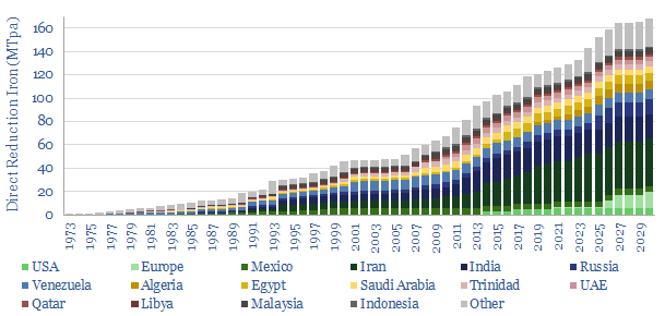
Direct reduced iron underpins 6% of global steel production, running to 120MTpa of the world 2GTpa global steel production and ramping up steadily since the 1970s (chart below).
How does the direct reduction iron process work? Iron ore is heated in a shaft furnace, alongside syngas, which contains CO and H2 derived from natural gas, thereby reducing the iron oxide, while forming waste gases of H2O and CO2. The product can later be upgraded into steel in an electric arc furnace.
Leading DRI technologies include Midrex and Tenova HYL, and the data-file contains a database of all the deployments to-date, plus future low-carbon plans.
DRI products include Hot DRI (converted straight into an EAF before it is cooled down), Cold DRI that is cooled down to below 60C before subsequent processing, and ‘Hot Briquetted Iron’ (HBI), which is a stabilized product and can be shipped globally in a bulk tanker.
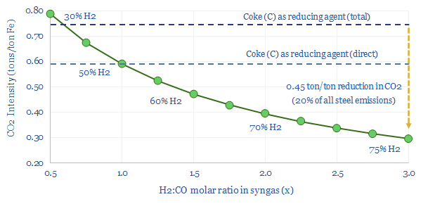
Base case costs for producing DRI most likely run to $300/ton of iron, to earn a 10% IRR on a 2MTpa production facility costing $600M. Energy intensity is most likely around 3,000 kWh/ton and CO2 intensity is modelled at 0.6 tons/ton of iron, although this will vary according to the percent of iron reduction delivered by hydrogen versus CO (chart below).
For decarbonization of the steel industry, we think that direct reduced iron can increasingly be made with hydrogen comprising almost all of the reducing agent, and renewables-heavy electricity. Ultimately, this can reduce the total CO2 intensity to 0.6 tons/ton, which is 75% below higher-CO2 steel.
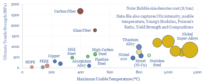
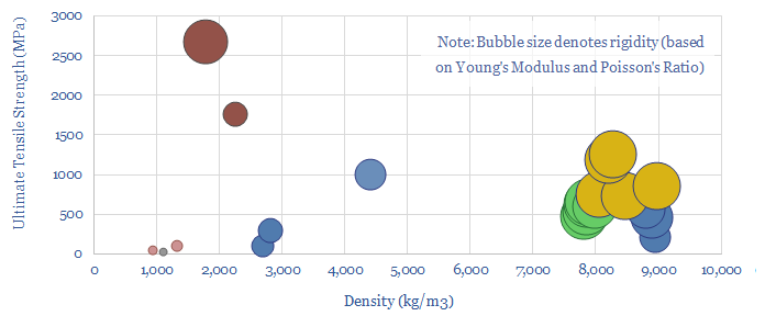
This data-file aggregates information into the strength, temperature resistance, rigidity, costs and CO2 intensities of important structural metals and materials. It shows why nickel-based super-alloys are used in gas turbines and jet engines; why glass fiber and carbon fiber are used in wind turbine blades; why traces of Rare Earth metals are introduced into high-pressure pipelines for gas transportation or CCS; why overhead power lines are blends of aluminium and steel.
Strength is the ability to withstand forces? 1 Pascal means that a force of 1 Newton is acting over an area of 1 m2. When applied to gases, 1 Pascal of force per m2 of area denotes pressure. But when applied to solid materials, 1 Pascal of force per m2 of area denotes stress.
Stress and strain. As more stress is applied to materials, they begin to deform. For example, under ‘tensile stress’, where the force is pulling a material apart, the strain may occur as elongation.
Elastic Deformation. The type of strain caused by low levels of tensile stress is ‘elastic deformation’, which means that the material will revert to its original shape when the stress is removed.
Young’s Modulus. During elastic deformation, there will be a fixed ratio of stress-to-strain. Each additional unit of stress (in GPa) causes a fixed degree of elongation (dimensionless). High Young’s Modulus means a more rigid and less elastic material.
Yield Strength. Beyond a certain degree of stress, additional stress will not cause further elastic deformation, but instead, will cause plastic deformation. When this stress is removed, then the material does not return to its original shape. Yield strength is measured in MPa.
Ultimate Tensile Strength. If stress increases further, then ultimately the material will fail. It will ‘neck open’ and then tear. The point at which this begins to happen is the Ultimate Tensile Strength. And it is also measured in MPa. In other words, a tensile strength of 500 MPa means that it will take a mass of 50kT tons to tear apart 1m2 of a material.
Poisson’s Ratio. Also during elastic deformation, as a material stretches, it will become narrower. A very stretchy material, such as rubber, has a Poisson’s Ratio close to 0.5. Conversely, a material such as paper has a very low Poisson’s Ratio, around 0.1, and will ‘give’ very little before tearing.
Other Metrics. There are other types of stress, such as compressive, shear and rotational stress. We are not going to catalogue all of these properties in this file, but use tensile stress as a proxy.
This data-file aggregates information into the strength, temperature resistance, rigidity, costs and CO2 intensities of important structural metals and materials, which matter increasingly in the energy transition.
The data show why nickel-based super-alloys are used in gas turbines and jet engines, due to their resistance to deformation, even at high temperatures. The efficiency of a gas turbine/jet engine is a direct function of the hottest temperature in the Brayton Cycle.
In CCS and gas transportation, traces of Rare Earth metals such as Niobium are introduced into high-pressure pipelines, to impart higher strength, and enable higher volumes of flow, even of mildly corrosive fluids, without requiring overly thick pipeline walls.
Biogas costs are broken down in this economic model, generating a 10% IRR off $180M/kboed capex, via a mixture of $16/mcfe gas sales, $60/ton waste disposal fees and $50/ton CO2 prices. High gas prices and landfill taxes can make biogas economical in select geographies. Although diseconomies of scale reward smaller projects?
Biogas is a mixture of 50-70% methane and 30-50% CO2, produced from the anaerobic digestion of organic matter, such as manure, sewage or crop residues, or other organic waste. Archaea notes that 72% of US renewable natural gas comes from landfills, 20% from livestock, 5% from organic waste and 3% from wastewater.
This economic model captures the costs of biogas production, informed by 20 case studies, covering yields, capex, opex, IRRs and sensitivities.
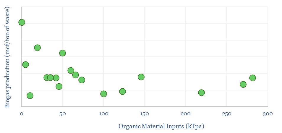
Biogas yields average around 4 mcf per ton of input material, although smaller plants may find it easier to source high-quality feedstocks, with greater quantities of volatile organic matter, and greater conversion of that matter into biogas (chart below).
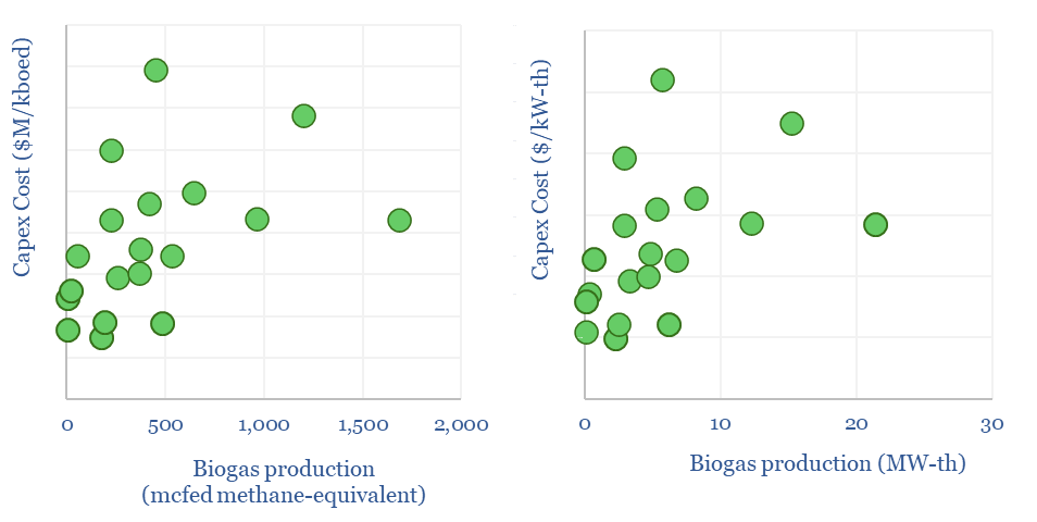
The capex costs of biogas plants are also tabulated from the 20 case studies in this data-file. Costs vary. But good rules of thumb might be $200/Tpa of feedstocks. In energy industry terms, this is equivalent to around $180M/kboed, or around 6x the costs of offshore hydrocarbons, or around $2,500/kW-th, which again is around 2x higher than the per kW-e costs of solar or onshore wind.
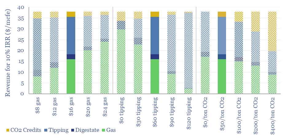
Biogas production facilities need to earn around $35-40/mcfe of methane-equivalent production in order to generate a 10% IRR on their up-front capex. There are four main revenue streams: gas, waste disposal fees, CO2 prices or incentives, and the value of residual digestate, which can be used as fertilizer or bedding in agriculture.
Our base case biogas cost model sees a 10% IRR from a combination of $16/mcf methane, $60/ton disposal fees and a $50/ton CO2 incentive. However, $120/ton landfill taxes can take the methane-equivalent price down to as little as $2.5/mcf. Hence the economics depend on landfill taxes and gas prices in different countries.
Biogas production in Europe currently comprises around 1-2% of the total gas grid, although some studies have estimated that total biogas production could reach 10-20% of total, or around 50-100bcm pa in Europe, via a “huge scale-up”.
One interesting observation from the charts above is that unlike other economic models in our library, biogas facilities may not benefit from economies of scale. Smaller facilities seem to cost less in capex terms and achieve higher yields. This suggests an opportunity for middle-markets private equity and companies with many small facilities?
Please download the data-file to stress-test biogas production costs. We are also constructive on some of the economic opportunities in landfill gas and biochar.
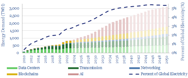
Powering the internet consumed 800 TWH of electricity in 2022, as 5bn users generated 4.7 Zettabytes of traffic. Our guess is that the internet’s energy demands double by 2030, including due to AI (e.g., ChatGPT), adding 1% upside to global energy demand and 2.5% to global electricity demand. This 14-page note aims to break down the numbers and their implications.
Cookies?
This website uses necessary cookies. Our cookies are simply to improve your experience. We do not undertake any advertising or targeting via our cookies. By clicking 'accept' or continuing to use the website, you consent to our use of cookies.AcceptRead More
Privacy & Cookies Policy
Privacy Overview
This website uses cookies to improve your experience while you navigate through the website. Out of these, the cookies that are categorized as necessary are stored on your browser as they are essential for the working of basic functionalities of the website. We also use third-party cookies that help us analyze and understand how you use this website. These cookies will be stored in your browser only with your consent. You also have the option to opt-out of these cookies. But opting out of some of these cookies may affect your browsing experience.
Necessary cookies are absolutely essential for the website to function properly. This category only includes cookies that ensures basic functionalities and security features of the website. These cookies do not store any personal information.
Any cookies that may not be particularly necessary for the website to function and is used specifically to collect user personal data via analytics, ads, other embedded contents are termed as non-necessary cookies. It is mandatory to procure user consent prior to running these cookies on your website.